# 九、用于 TensorFlow Eager 時間序列回歸的遞歸神經網絡 大家好！ 在本教程中，我們將探討如何為時間序列回歸構建循環神經網絡。 由于我的背景在電力系統中，我認為最好包括該領域相關的教程。 因此，在本教程中，我們將構建一個用于能源需求預測的 RNN。 為了預測第二天的能源需求，我們將使用 ENTSO-E 提供的每小時能耗數據。 我選擇使用來自西班牙的數據，因為我目前住在這里。 然而，相同的分析可以應用于來自任何國家的能耗數據。 教程步驟  + ENTSO-E 能源需求數據的探索性數據分析 + 創建訓練和測試數據集 + 處理原始數據來創建輸入和標簽樣本 + 為回歸創建 RNN 類 + 從頭開始或從以前的檢查點使用梯度下降訓練模型 + 展示測試集上的預測值和實際值之間的差異 如果你想在本教程中添加任何內容，請告訴我們。 此外，我很高興聽到你的任何改進建議。 ## 導入有用的庫 ```py # 導入 TensorFlow 和 TensorFlow Eager import tensorflow.contrib.eager as tfe import tensorflow as tf # 導入用于數據處理的庫 from sklearn.preprocessing import StandardScaler from datetime import datetime as dt import pandas as pd import numpy as np # 導入繪圖庫 import matplotlib.pyplot as plt %matplotlib inline # 開啟 Eager 模式。一旦開啟不能撤銷！只執行一次。 tfe.enable_eager_execution(device_policy=tfe.DEVICE_PLACEMENT_SILENT) ``` ## 探索性數據分析 可以在文件夾datasets / load_forecasting中找到本教程中使用的數據集。 我們讀取它，來看看吧！ ```py energy_df = pd.read_csv('datasets/load_forecasting/spain_hourly_entsoe.csv') energy_df.tail(2) ``` | | Time (CET) | Day-ahead Total Load Forecast [MW] - BZN|ES | Actual Total Load [MW] - BZN|ES | | --- | --- | --- | --- | | 29230 | 02.05.2018 22:00 - 02.05.2018 23:00 | 30187.0 | 30344.0 | | 29231 | 02.05.2018 23:00 - 03.05.2018 00:00 | 27618.0 | 27598.0 | ```py # 重命名行 energy_df.columns = ['time', 'forecasted_load', 'actual_load'] # 從 'Time (CET)' 中提取日期和時間 energy_df['date'] = energy_df['time'].apply(lambda x: dt.strptime(x.split('-')[0].strip(), '%d.%m.%Y %H:%M')) ``` 如你所見，數據集附帶每個測量的時間戳，特定小時的實際能量需求，以及預測值。 對于我們的任務，我們只使用`Actual Total Load [MW]`列。 ```py printprint(('The date of the first measurement: ''The da , energy_df.loc[0, 'time']) # The date of the first measurement: 01.01.2015 00:00 - 01.01.2015 01:00 print('The date of the last measurement: ', energy_df.loc[len(energy_df)-1, 'time']) # The date of the last measurement: 02.05.2018 23:00 - 03.05.2018 00:00 ``` 該數據集包括從 2015 年 1 月 1 日到 2018 年 5 月 2 日的每小時能耗數據。最近的數據！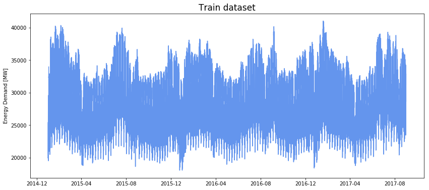 ## 從時間序列數據創建輸入和標簽樣本 ### 將數據分割為訓練/測試數據集 數據處理的第一步是從原始數據創建訓練和測試數據集。 我選擇將 80% 的數據保留在訓練集中，20% 保留在測試集中。 通過修改`train_size`變量，隨意調整此參數。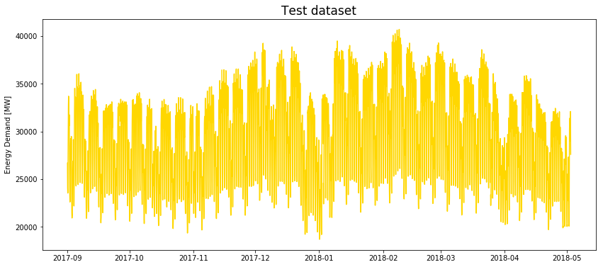 ```py # 將數據分割為訓練和測試數據集 train_size = 0.8 end_train = int(len(energy_df)*train_size/24)*24 train_energy_df = energy_df.iloc[:end_train,:] test_energy_df = energy_df.iloc[end_train:,:] # 繪制訓練集 plt.figure(figsize=(14,6)) plt.plot(train_energy_df['date'], train_energy_df['actual_load'], color='cornflowerblue'); plt.title('Train dataset', fontsize=17); plt.ylabel('Energy Demand [MW]'); ```  ```py # 繪制測試集 plt.figure(figsize=(14,6)) plt.plot(test_energy_df['date'], test_energy_df['actual_load'], color='gold'); plt.title('Test dataset', fontsize=17); plt.ylabel('Energy Demand [MW]'); ```  ### 縮放數據集 數據被標準化后，神經網絡工作得更好，收斂速度更快。 對于此任務，我選擇使用零均值和單位方差對數據進行標準化，因為我發現這對 LSTM 更有效。 你還可以嘗試使用`MinMaxScaler`對數據進行標準化，看看是否可以獲得更好的結果。 ```py # 為缺失的度量進行差值 train_energy_df = train_energy_df.interpolate(limit_direction='both') test_energy_df = test_energy_df.interpolate(limit_direction='both') scaler = StandardScaler().fit(train_energy_df['actual_load'][:,None]) train_energy_df['actual_load'] = scaler.transform(train_energy_df['actual_load'][:,None]) test_energy_df['actual_load'] = scaler.transform(test_energy_df['actual_load'][:,None]) ``` ### 創建滑動窗口樣本 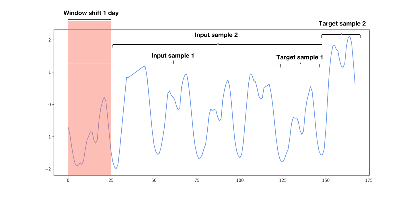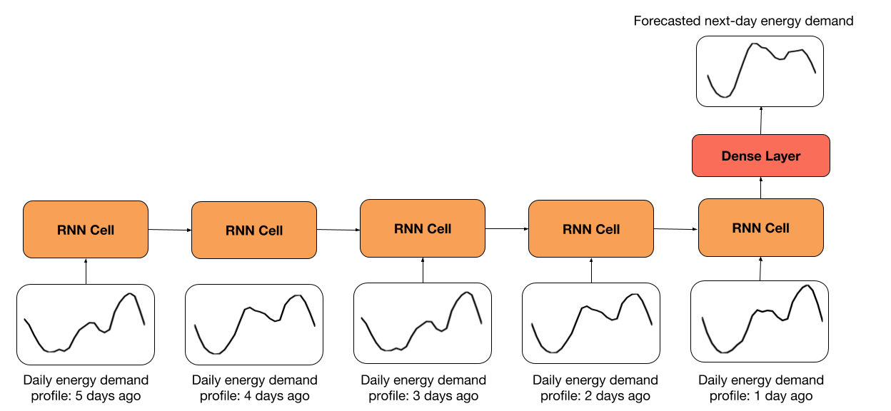你可以在我創建的函數下面的代碼單元格中找到，從時間序列數據生成輸入和標簽樣本。 每個 RNN 單元中的輸入是一天的每小時數據。 時間步數由`look_back`變量定義，該變量指定要回顧的天數。 默認值為 5 天，這意味著 RNN 將展開 5 個步驟。 你還可以指定預測的天數，默認為一天。 輸入和標簽樣本是基于`look_back`和`predict_ahead`變量創建的，如下圖所示。  ```py def moving_window_samples(timeseries, look_back=5, predict_ahead=1): ''' 用于從時間序列創建輸入和標簽樣本的函數，延遲為一天。 Args: timeseries: timeseries dataset. look_back: the size of the input. Specifies how many days to look back. predict_ahead: size of the output. Specifies how many days to predict ahead. Returns: input_samples: the input samples createad from the timeseries, using a window shift of one day. target_samples: the target corresponding to each input sample. ''' n_strides = int((len(timeseries)- predict_ahead*24 - look_back*24 + 24)/24) input_samples = np.zeros((n_strides, look_back*24)) target_samples = np.zeros((n_strides, predict_ahead*24)) for i in range(n_strides): end_input = i*24 + look_back*24 input_samples[i,:] = timeseries[i*24:end_input] target_samples[i,:] = timeseries[end_input:(end_input + predict_ahead*24)] # 將輸入形狀修改為（樣本數，時間步長，輸入維度） input_samples = input_samples.reshape((-1, look_back, 24)) return input_samples.astype('float32'), target_samples.astype('float32') train_input_samples, train_target_samples = moving_window_samples(train_energy_df['actual_load'], look_back=5, predict_ahead=1) test_input_samples, test_target_samples = moving_window_samples(test_energy_df['actual_load'], look_back=5, predict_ahead=1) ``` ### 使用`tf.data.Dataset`創建訓練和測試數據集 通常，我們使用`tf.data.Dataset` API 將數據傳輸到張量。 我選擇了 64 的批量大小，但隨意調整它。 在訓練網絡時，我們可以使用`tfe.Iterator`函數非常輕松地遍歷這些數據集。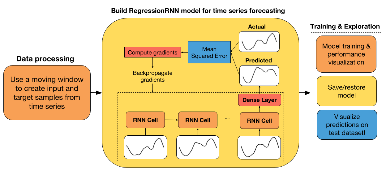 ```py # 隨意修改批量大小 # 通常較小的批量大小在測試集上獲得更好的結果 batch_size = 64 train_dataset = (tf.data.Dataset.from_tensor_slices( (train_input_samples, train_target_samples)).batch(batch_size)) test_dataset = (tf.data.Dataset.from_tensor_slices( (test_input_samples, test_target_samples)).batch(batch_size)) ``` ## 兼容 Eager API 的 RNN 回歸模型 RNN 模型的類與以前的模型非常相似。 在初始化期間，我們定義了正向傳播中所需的所有層。 我們還可以指定要在其上執行計算的設備，以及我們希望恢復或保存模型變量的文件路徑。 該模型繼承自`tf.keras.Model`，以便跟蹤所有變量。 該模型的架構非常簡單。 我們只需獲取最后`look_back`天的每小時數據，然后將其傳給 RNN。 最終輸出傳給了帶有 ReLU 激活的密集層。 輸出層大小由`predict_ahead`變量定義。 在我們的例子中，輸出大小是 24 個單元，因為我們預測第二天的能源需求。  ```py class RegressionRNN(tf.keras.Model): def __init__(self, cell_size=64, dense_size=128, predict_ahead=1, device='cpu:0', checkpoint_directory=None): ''' 定義在正向傳播期間使用的參數化層，你要在上面運行計算的設備以及檢查點目錄。 另外，你還可以修改網絡的默認大小。 Args: cell_size: RNN cell size. dense_size: the size of the dense layer. predict_ahead: the number of days you would like to predict ahead. device: string, 'cpu:n' or 'gpu:n' (n can vary). Default, 'cpu:0'. checkpoint_directory: the directory where you would like to save/restore a model. ''' super(RegressionRNN, self).__init__() # 權重初始化函數 w_initializer = tf.contrib.layers.xavier_initializer() # 偏置初始化函數 b_initializer = tf.zeros_initializer() # 密集層初始化 self.dense_layer = tf.keras.layers.Dense(dense_size, activation=tf.nn.relu, kernel_initializer=w_initializer, bias_initializer=b_initializer) # 預測層初始化 self.pred_layer = tf.keras.layers.Dense(predict_ahead*24, activation=None, kernel_initializer=w_initializer, bias_initializer=b_initializer) # 基本的 LSTM 單元 self.rnn_cell = tf.nn.rnn_cell.BasicLSTMCell(cell_size) # 定義設備 self.device = device # 定義檢查點目錄 self.checkpoint_directory = checkpoint_directory def predict(self, X): ''' 在網絡上執行正向傳播 Args: X: 3D tensor of shape (batch_size, timesteps, input_dimension). Returns: preds: the final predictions of the network. ''' # 獲取一個批量的樣本數量 num_samples = tf.shape(X)[0] # 初始化 LSTM 單元狀態為零 state = self.rnn_cell.zero_state(num_samples, dtype=tf.float32) # 分割輸入 unstacked_input = tf.unstack(X, axis=1) # 遍歷每個時間步驟 for input_step in unstacked_input: output, state = self.rnn_cell(input_step, state) # 將最后一個單元狀態傳給密集層（ReLU 激活） dense = self.dense_layer(output) # 計算最終的預測 preds = self.pred_layer(dense) return preds def loss_fn(self, X, y): """ 定義訓練期間使用的損失函數 """ preds = self.predict(X) loss = tf.losses.mean_squared_error(y, preds) return loss def grads_fn(self, X, y): """ 在每個正向步驟中， 動態計算損失值對模型參數的梯度 """ with tfe.GradientTape() as tape: loss = self.loss_fn(X, y) return tape.gradient(loss, self.variables) def restore_model(self): """ 用于恢復訓練模型的函數 """ with tf.device(self.device): # 運行模型一次來初始化變量 dummy_input = tf.constant(tf.zeros((1, 5, 24))) dummy_pred = self.predict(dummy_input) # 恢復模型變量 saver = tfe.Saver(self.variables) saver.restore(tf.train.latest_checkpoint (self.checkpoint_directory)) def save_model(self, global_step=0): """ 用于保存訓練模型的函數 """ tfe.Saver(self.variables).save(self.checkpoint_directory, global_step=global_step) def fit(self, training_data, eval_data, optimizer, num_epochs=500, early_stopping_rounds=10, verbose=10, train_from_scratch=False): """ 用于訓練模型的函數， 使用所選的優化器，執行所需數量的迭代 你可以從零開始訓練，或者加載最后訓練的模型 使用了提前停止來降低網絡的過擬合風險 Args: training_data: the data you would like to train the model on. Must be in the tf.data.Dataset format. eval_data: the data you would like to evaluate the model on. Must be in the tf.data.Dataset format. optimizer: the optimizer used during training. num_epochs: the maximum number of iterations you would like to train the model. early_stopping_rounds: stop training if the loss on the eval dataset does not decrease after n epochs. verbose: int. Specify how often to print the loss value of the network. train_from_scratch: boolean. Whether to initialize variables of the the last trained model or initialize them randomly. """ if train_from_scratch==False: self.restore_model() # 初始化最佳損失。這個遍歷儲存評估數據集上的最低損失 best_loss = 999 # 初始化類別來更新訓練和評估平均損失 train_loss = tfe.metrics.Mean('train_loss') eval_loss = tfe.metrics.Mean('eval_loss') # 初始化目錄來儲存損失歷史 self.history = {} self.history['train_loss'] = [] self.history['eval_loss'] = [] # 開始訓練 with tf.device(self.device): for i in range(num_epochs): # 使用梯度下降來訓練 for X, y in tfe.Iterator(training_data): grads = self.grads_fn(X, y) optimizer.apply_gradients(zip(grads, self.variables)) # 計算一個迭代后訓練數據上的損失 for X, y in tfe.Iterator(training_data): loss = self.loss_fn(X, y) train_loss(loss) self.history['train_loss'].append(train_loss.result().numpy()) # 重置指標 train_loss.init_variables() # 計算一個迭代后評估數據上的損失 for X, y in tfe.Iterator(eval_data): loss = self.loss_fn(X, y) eval_loss(loss) self.history['eval_loss'].append(eval_loss.result().numpy()) # 重置指標 eval_loss.init_variables() # 打印訓練和評估損失 if (i==0) | ((i+1)%verbose==0): print('Train loss at epoch %d: ' %(i+1), self.history['train_loss'][-1]) print('Eval loss at epoch %d: ' %(i+1), self.history['eval_loss'][-1]) # 為提前停止而檢查 if self.history['eval_loss'][-1]<best_loss: best_loss = self.history['eval_loss'][-1] count = early_stopping_rounds else: count -= 1 if count==0: break ``` ## 使用梯度下降來訓練模型 ```py # 指定你打算保存/恢復訓練變量的路徑 checkpoint_directory = 'models_checkpoints/DemandRNN/' # 如果可用，則使用 GPU device = 'gpu:0' if tfe.num_gpus()>0 else 'cpu:0' # 定義優化器 optimizer = tf.train.AdamOptimizer(learning_rate=1e-2) # 實例化模型。這并不會實例化變量。 model = RegressionRNN(cell_size=16, dense_size=16, predict_ahead=1, device=device, checkpoint_directory=checkpoint_directory) # 訓練模型 model.fit(train_dataset, test_dataset, optimizer, num_epochs=500, early_stopping_rounds=5, verbose=50, train_from_scratch=True) ''' Train loss at epoch 1: 0.5420932229608297 Eval loss at epoch 1: 0.609554298222065 Train loss at epoch 50: 0.024180740118026733 Eval loss at epoch 50: 0.049175919964909554 ''' # 保存模型 model.save_model() ``` ## 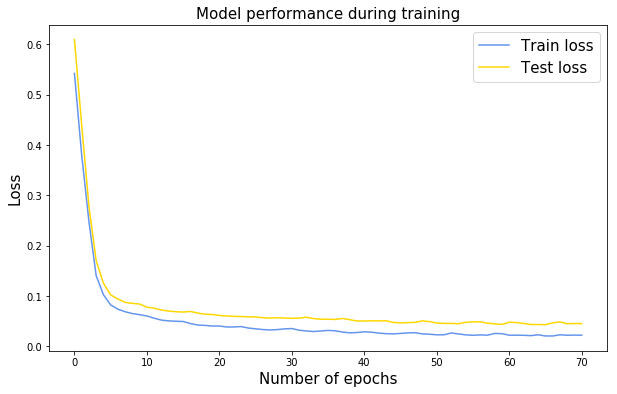在訓練期間展示表現 我們可以很容易地看到在模型擬合過程中自動跟蹤的損失歷史。 ```py plt.figure(figsize=(10, 6)) plt.plot(range(len(model.history['train_loss'])), model.history['train_loss'], color='cornflowerblue', label='Train loss'); plt.plot(range(len(model.history['eval_loss'])), model.history['eval_loss'], color='gold', label='Test loss'); plt.title('Model performance during training', fontsize=15) plt.xlabel('Number of epochs', fontsize=15); plt.ylabel('Loss', fontsize=15); plt.legend(fontsize=15); ```  ## 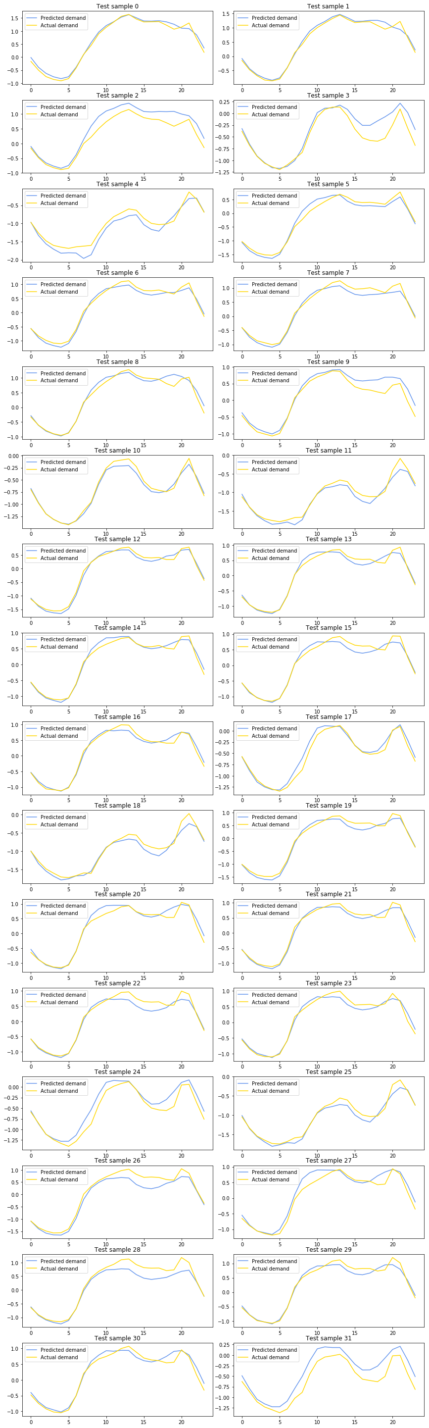展示測試集上的預測 這是本教程的最后一部分。 在對網絡進行訓練后，我們可以可展示測試數據集進行的預測。 如果你已經跳過訓練，我添加了一個單元格，你可以輕松恢復已經訓練過的模型。 ```py ################################################## # 恢復之前訓練過的模型 ################################################## tf.reset_default_graph() checkpoint_directory = 'models_checkpoints/DemandRNN/' model = RegressionRNN(cell_size=16, dense_size=16, predict_ahead=1, device=device, checkpoint_directory=checkpoint_directory) model.restore_model() # INFO:tensorflow:Restoring parameters from models_checkpoints/DemandRNN/-0 ################################################### # 展示實際值和預測值 ################################################### with tf.device(device): # 創建輸入和標簽樣本的迭代器 X_test, y_test = tfe.Iterator(test_dataset).next() # 預測測試批量 preds = model.predict(X_test).numpy() y = y_test.numpy() # 為一般的批量樣本（32）創建子圖 f, axarr = plt.subplots(16, 2, figsize=(12, 40)) f.tight_layout() # 繪制預測 i, j = 0, 0 for idx in range(32): axarr[i,j].plot(range(24), preds[idx,:], label='Predicted demand', color='cornflowerblue') axarr[i,j].plot(range(24), y[idx,:], label='Actual demand', color='gold') axarr[i,j].legend() axarr[i,j].set_title('Test sample %d' %idx) if j==1: i += 1 j = 0 else: j += 1 ```