六、神經網絡 · ApacheCN 深度學習譯文集

# 六、神經網絡在本章中，我們將介紹神經網絡以及如何在 TensorFlow 中實現它們。大多數后續章節將基于神經網絡，因此學習如何在 TensorFlow 中使用它們非常重要。在開始使用多層網絡之前，我們將首先介紹神經網絡的基本概念。在上一節中，我們將創建一個神經網絡，學習如何玩井字棋。在本章中，我們將介紹以下秘籍： * 實現操作門 * 使用門和激活函數 * 實現單層神經網絡 * 實現不同的層 * 使用多層網絡 * 改進線性模型的預測 * 學習玩井字棋讀者可以在 [Github](https://github.com/nfmcclure/tensorflow_cookbook) 和[ Packt 倉庫](https://github.com/PacktPublishing/TensorFlow-Machine-Learning-Cookbook-Second-Edition)中找到本章中的所有代碼。 # 介紹神經網絡目前在諸如圖像和語音識別，閱讀手寫，理解文本，圖像分割，對話系統，自動駕駛汽車等任務中打破記錄。雖然這些上述任務中的一些將在后面的章節中介紹，但重要的是將神經網絡作為一種易于實現的機器學習算法引入，以便我們以后可以對其進行擴展。神經網絡的概念已經存在了幾十年。然而，它最近才獲得牽引力，因為我們現在具有訓練大型網絡的計算能力，因為處理能力，算法效率和數據大小的進步。神經網絡基本上是應用于輸入數據矩陣的一系列操作。這些操作通常是加法和乘法的集合，然后是非線性函數的應用。我們已經看到的一個例子是邏輯回歸，我們在第 3 章，線性回歸中看到了這一點。邏輯回歸是部分斜率 - 特征乘積的總和，其后是應用 Sigmoid 函數，這是非線性的。神經網絡通過允許操作和非線性函數的任意組合（包括絕對值，最大值，最小值等的應用）來進一步概括這一點。神經網絡的重要技巧稱為反向傳播。反向傳播是一種允許我們根據學習率和損失函數輸出更新模型變量的過程。我們使用反向傳播來更新第 3 章，線性回歸和第 4 章，支持向量機中的模型變量。關于神經網絡的另一個重要特征是非線性激活函數。由于大多數神經網絡只是加法和乘法運算的組合，因此它們無法對非線性數據集進行建模。為了解決這個問題，我們在神經網絡中使用了非線性激活函數。這將允許神經網絡適應大多數非線性情況。重要的是要記住，正如我們在許多算法中所看到的，神經網絡對我們選擇的超參數敏感。在本章中，我們將探討不同學習率，損失函數和優化程序的影響。 > 學習神經網絡的資源更多，更深入，更詳細地涵蓋了該主題。這些資源如下： * [描述反向傳播的開創性論文是 Yann LeCun 等人的 Efficient Back Prop](http://yann.lecun.com/exdb/publis/pdf/lecun-98b.pdf) * [CS231，用于視覺識別的卷積神經網絡，由斯坦福大學提供。](http://cs231n.stanford.edu/) * [CS224d，斯坦福大學自然語言處理的深度學習。](http://cs224d.stanford.edu/) * [深度學習，麻省理工學院出版社出版的一本書，Goodfellow 等人，2016]http://www.deeplearningbook.org)。 * 邁克爾·尼爾森（Michael Nielsen）有一本名為[“神經網絡與深度學習”](http://neuralnetworksanddeeplearning.com/)的在線書籍。 * 對于一個更實用的方法和神經網絡的介紹，Andrej Karpathy 用 JavaScript 實例寫了一個很棒的總結，稱為[黑客的神經網絡指南](http://karpathy.github.io/neuralnets/)。 * 另一個總結深度學習的網站被 Ian Goodfellow，Yoshua Bengio 和 Aaron Courville 稱為[初學者深度學習](http://randomekek.github.io/deep/deeplearning.html)。 # 實現操作門神經網絡最基本的概念之一是作為操作門操作。在本節中，我們將從乘法操作開始作為門，然后再繼續考慮嵌套門操作。 ## 準備我們將實現的第一個操作門是`f(x) = a · x`。為優化此門，我們將`a`輸入聲明為變量，將`x`輸入聲明為占位符。這意味著 TensorFlow 將嘗試更改`a`值而不是`x`值。我們將創建損失函數作為輸出和目標值之間的差異，即 50。第二個嵌套操作門將是`f(x) = a · x + b`。同樣，我們將`a`和`b`聲明為變量，將`x`聲明為占位符。我們再次將輸出優化到目標值 50。值得注意的是，第二個例子的解決方案并不是唯一的。有許多模型變量組合可以使輸出為 50.對于神經網絡，我們并不關心中間模型變量的值，而是更加強調所需的輸出。將這些操作視為我們計算圖上的操作門。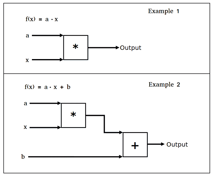下圖描繪了前面兩個示例： ![](https://img.kancloud.cn/d5/c9/d5c96c6aacd54897fc3036297dfbd344_874x724.png) 圖 1：本節中的兩個操作門示例 ## 操作步驟要在 TensorFlow 中實現第一個操作門`f(x) = a · x`并將輸出訓練為值 50，請按照下列步驟操作： 1. 首先加載`TensorFlow`并創建圖會話，如下所示： ```py import tensorflow as tf sess = tf.Session() ``` 1. 現在我們需要聲明我們的模型變量，輸入數據和占位符。我們使輸入數據等于值`5`，因此得到 50 的乘法因子將為 10（即`5X10=50`），如下所示： ```py a = tf.Variable(tf.constant(4.)) x_val = 5. x_data = tf.placeholder(dtype=tf.float32) ``` 1. 接下來，我們使用以下輸入將操作添加到計算圖中： ```py multiplication = tf.multiply(a, x_data) ``` 1. 我們現在將損失函數聲明為輸出與`50`的期望目標值之間的 L2 距離，如下所示： ```py loss = tf.square(tf.subtract(multiplication, 50.)) ``` 1. 現在我們初始化我們的模型變量并將我們的優化算法聲明為標準梯度下降，如下所示： ```py init = tf.global_variables_initializer() sess.run(init) my_opt = tf.train.GradientDescentOptimizer(0.01) train_step = my_opt.minimize(loss) ``` 1. 我們現在可以將模型輸出優化到`50`的期望值。我們通過連續輸入 5 的輸入值并反向傳播損失來將模型變量更新為`10`的值，如下所示： ```py print('Optimizing a Multiplication Gate Output to 50.') for i in range(10): sess.run(train_step, feed_dict={x_data: x_val}) a_val = sess.run(a) mult_output = sess.run(multiplication, feed_dict={x_data: x_val}) print(str(a_val) + ' * ' + str(x_val) + ' = ' + str(mult_output)) ``` 1. 上一步應該產生以下輸出： ```py Optimizing a Multiplication Gate Output to 50\. 7.0 * 5.0 = 35.0 8.5 * 5.0 = 42.5 9.25 * 5.0 = 46.25 9.625 * 5.0 = 48.125 9.8125 * 5.0 = 49.0625 9.90625 * 5.0 = 49.5312 9.95312 * 5.0 = 49.7656 9.97656 * 5.0 = 49.8828 9.98828 * 5.0 = 49.9414 9.99414 * 5.0 = 49.9707 ``` 接下來，我們將對兩個嵌套的操作門`f(x) = a · x + b`進行相同的操作。 1. 我們將以與前面示例完全相同的方式開始，但將初始化兩個模型變量`a`和`b`，如下所示： ```py from tensorflow.python.framework import ops ops.reset_default_graph() sess = tf.Session() a = tf.Variable(tf.constant(1.)) b = tf.Variable(tf.constant(1.)) x_val = 5\. x_data = tf.placeholder(dtype=tf.float32) two_gate = tf.add(tf.multiply(a, x_data), b) loss = tf.square(tf.subtract(two_gate, 50.)) my_opt = tf.train.GradientDescentOptimizer(0.01) train_step = my_opt.minimize(loss) init = tf.global_variables_initializer() sess.run(init) ``` 1. 我們現在優化模型變量以將輸出訓練到`50`的目標值，如下所示： ```py print('Optimizing Two Gate Output to 50.') for i in range(10): # Run the train step sess.run(train_step, feed_dict={x_data: x_val}) # Get the a and b values a_val, b_val = (sess.run(a), sess.run(b)) # Run the two-gate graph output two_gate_output = sess.run(two_gate, feed_dict={x_data: x_val}) print(str(a_val) + ' * ' + str(x_val) + ' + ' + str(b_val) + ' = ' + str(two_gate_output)) ``` 1. 上一步應該產生以下輸出： ```py Optimizing Two Gate Output to 50\. 5.4 * 5.0 + 1.88 = 28.88 7.512 * 5.0 + 2.3024 = 39.8624 8.52576 * 5.0 + 2.50515 = 45.134 9.01236 * 5.0 + 2.60247 = 47.6643 9.24593 * 5.0 + 2.64919 = 48.8789 9.35805 * 5.0 + 2.67161 = 49.4619 9.41186 * 5.0 + 2.68237 = 49.7417 9.43769 * 5.0 + 2.68754 = 49.876 9.45009 * 5.0 + 2.69002 = 49.9405 9.45605 * 5.0 + 2.69121 = 49.9714 ``` > 這里需要注意的是，第二個例子的解決方案并不是唯一的。這在神經網絡中并不重要，因為所有參數都被調整為減少損失。這里的最終解決方案將取決于`a`和`b`的初始值。如果這些是隨機初始化的，而不是值 1，我們會看到每次迭代的模型變量的不同結束值。 ## 工作原理我們通過 TensorFlow 的隱式反向傳播實現了計算門的優化。 TensorFlow 跟蹤我們的模型的操作和變量值，并根據我們的優化算法規范和損失函數的輸出進行調整。我們可以繼續擴展操作門，同時跟蹤哪些輸入是變量，哪些輸入是數據。這對于跟蹤是很重要的，因為 TensorFlow 將更改所有變量以最小化損失而不是數據，這被聲明為占位符。每個訓練步驟自動跟蹤計算圖并自動更新模型變量的隱式能力是 TensorFlow 的強大功能之一，也是它如此強大的原因之一。 # 使用門和激活函數現在我們可以將操作門連接在一起，我們希望通過激活函數運行計算圖輸出。在本節中，我們將介紹常見的激活函數。 ## 準備在本節中，我們將比較和對比兩種不同的激活函數：Sigmoid 和整流線性單元（ReLU）。回想一下，這兩個函數由以下公式給出： ![](https://img.kancloud.cn/9a/38/9a383d6541cf310dd20d94b62f74741e_2330x420.png) ![](https://img.kancloud.cn/ec/20/ec2042e962bd1a7534e3d1e55a7a066c_1770x210.png) 在這個例子中，我們將創建兩個具有相同結構的單層神經網絡，除了一個將通過 sigmoid 激活并且一個將通過 ReLU 激活。損失函數將由距離值 0.75 的 L2 距離控制。我們將從正態分布`(Normal(mean=2, sd=0.1))`中隨機抽取批量數據，然后將輸出優化為 0.75。 ## 操作步驟我們按如下方式處理秘籍： 1. 我們將首先加載必要的庫并初始化圖。這也是我們可以提出如何使用 TensorFlow 設置隨機種子的好點。由于我們將使用 NumPy 和 TensorFlow 中的隨機數生成器，因此我們需要為兩者設置隨機種子。使用相同的隨機種子集，我們應該能夠復制結果。我們通過以下輸入執行此操作： ```py import tensorflow as tf import numpy as np import matplotlib.pyplot as plt sess = tf.Session() tf.set_random_seed(5) np.random.seed(42) ``` 1. 現在我們需要聲明我們的批量大小，模型變量，數據和占位符來輸入數據。我們的計算圖將包括將我們的正態分布數據輸入到兩個相似的神經網絡中，這兩個神經網絡的區別僅在于激活函數。結束，如下所示： ```py batch_size = 50 a1 = tf.Variable(tf.random_normal(shape=[1,1])) b1 = tf.Variable(tf.random_uniform(shape=[1,1])) a2 = tf.Variable(tf.random_normal(shape=[1,1])) b2 = tf.Variable(tf.random_uniform(shape=[1,1])) x = np.random.normal(2, 0.1, 500) x_data = tf.placeholder(shape=[None, 1], dtype=tf.float32) ``` 1. 接下來，我們將聲明我們的兩個模型，即 sigmoid 激活模型和 ReLU 激活模型，如下所示： ```py sigmoid_activation = tf.sigmoid(tf.add(tf.matmul(x_data, a1), b1)) relu_activation = tf.nn.relu(tf.add(tf.matmul(x_data, a2), b2)) ``` 1. 損失函數將是模型輸出與值 0.75 之間的平均 L2 范數，如下所示： ```py loss1 = tf.reduce_mean(tf.square(tf.subtract(sigmoid_activation, 0.75))) loss2 = tf.reduce_mean(tf.square(tf.subtract(relu_activation, 0.75))) ``` 1. 現在我們需要聲明我們的優化算法并初始化我們的變量，如下所示： ```py my_opt = tf.train.GradientDescentOptimizer(0.01) train_step_sigmoid = my_opt.minimize(loss1) train_step_relu = my_opt.minimize(loss2) init = tf.global_variable_initializer() sess.run(init) ``` 1. 現在，我們將針對兩個模型循環我們的 750 次迭代訓練，如下面的代碼塊所示。我們還將保存損失輸出和激活輸出值，以便稍后進行繪圖： ```py loss_vec_sigmoid = [] loss_vec_relu = [] activation_sigmoid = [] activation_relu = [] for i in range(750): rand_indices = np.random.choice(len(x), size=batch_size) x_vals = np.transpose([x[rand_indices]]) sess.run(train_step_sigmoid, feed_dict={x_data: x_vals}) sess.run(train_step_relu, feed_dict={x_data: x_vals}) loss_vec_sigmoid.append(sess.run(loss1, feed_dict={x_data: x_vals})) loss_vec_relu.append(sess.run(loss2, feed_dict={x_data: x_vals})) activation_sigmoid.append(np.mean(sess.run(sigmoid_activation, feed_dict={x_data: x_vals}))) activation_relu.append(np.mean(sess.run(relu_activation, feed_dict={x_data: x_vals}))) ``` 1. 要繪制損失和激活輸出，我們需要輸入以下代碼： ```py plt.plot(activation_sigmoid, 'k-', label='Sigmoid Activation') plt.plot(activation_relu, 'r--', label='Relu Activation') plt.ylim([0, 1.0]) plt.title('Activation Outputs') plt.xlabel('Generation') plt.ylabel('Outputs') plt.legend(loc='upper right') plt.show() plt.plot(loss_vec_sigmoid, 'k-', label='Sigmoid Loss') plt.plot(loss_vec_relu, 'r--', label='Relu Loss') plt.ylim([0, 1.0]) plt.title('Loss per Generation') plt.xlabel('Generation') plt.ylabel('Loss') plt.legend(loc='upper right') plt.show() ``` 激活輸出需要繪制，如下圖所示： ![](https://img.kancloud.cn/9a/ac/9aac9c61e9ddb34738ff359839d7caf8_393x281.png) 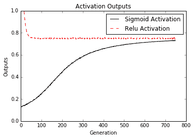圖 2：來自具有 Sigmoid 激活的網絡和具有 ReLU 激活的網絡的計算圖輸出兩個神經網絡使用類似的架構和目標（0.75），但有兩個不同的激活函數，sigmoid 和 ReLU。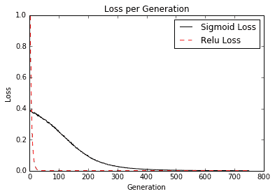重要的是要注意 ReLU 激活網絡收斂到比 sigmoid 激活所需的 0.75 目標更快，如下圖所示： ![](https://img.kancloud.cn/d9/78/d978a0bc83c18c20c8c34b3ca92966f3_393x281.png) 圖 3：該圖描繪了 Sigmoid 和 ReLU 激活網絡的損耗值。注意迭代開始時 ReLU 損失的極端程度 ## 工作原理由于 ReLU 激活函數的形式，它比 sigmoid 函數更頻繁地返回零值。我們認為這種行為是一種稀疏性。這種稀疏性導致收斂速度加快，但失去了受控梯度。另一方面，Sigmoid 函數具有非常良好控制的梯度，并且不會冒 ReLU 激活所帶來的極值的風險，如下圖所示： | 激活函數 | 優點 | 缺點 | | --- | --- | --- | | Sigmoid | 不太極端的輸出 | 收斂速度較慢 | | RELU | 更快地收斂 | 可能有極端的輸出值 | ## 更多在本節中，我們比較了神經網絡的 ReLU 激活函數和 Sigmoid 激活函數。還有許多其他激活函數通常用于神經網絡，但大多數屬于兩個類別之一；第一類包含形狀類似于 sigmoid 函數的函數，如 arctan，hypertangent，heavyiside step 等；第二類包含形狀的函數，例如 ReLU 函數，例如 softplus，leaky ReLU 等。我們在本節中討論的關于比較這兩個函數的大多數內容都適用于任何類別的激活。然而，重要的是要注意激活函數的選擇對神經網絡的收斂和輸出有很大影響。 # 實現單層神經網絡我們擁有實現對真實數據進行操作的神經網絡所需的所有工具，因此在本節中我們將創建一個神經網絡，其中一個層在`Iris`數據集上運行。 ## 準備在本節中，我們將實現一個具有一個隱藏層的神經網絡。重要的是要理解完全連接的神經網絡主要基于矩陣乘法。因此，重要的是數據和矩陣的大小正確排列。由于這是一個回歸問題，我們將使用均方誤差作為損失函數。 ## 操作步驟我們按如下方式處理秘籍： 1. 要創建計算圖，我們首先加載以下必要的庫： ```py import matplotlib.pyplot as plt import numpy as np import tensorflow as tf from sklearn import datasets ``` 1. 現在我們將加載`Iris`數據并將長度存儲為目標值。然后我們將使用以下代碼啟動圖會話： ```py iris = datasets.load_iris() x_vals = np.array([x[0:3] for x in iris.data]) y_vals = np.array([x[3] for x in iris.data]) sess = tf.Session() ``` 1. 由于數據集較小，我們需要設置種子以使結果可重現，如下所示： ```py seed = 2 tf.set_random_seed(seed) np.random.seed(seed) ``` 1. 為了準備數據，我們將創建一個 80-20 訓練測試分割，并通過最小 - 最大縮放將 x 特征標準化為 0 到 1 之間，如下所示： ```py train_indices = np.random.choice(len(x_vals), round(len(x_vals)*0.8), replace=False) test_indices = np.array(list(set(range(len(x_vals))) - set(train_indices))) x_vals_train = x_vals[train_indices] x_vals_test = x_vals[test_indices] y_vals_train = y_vals[train_indices] y_vals_test = y_vals[test_indices] def normalize_cols(m): col_max = m.max(axis=0) col_min = m.min(axis=0) return (m-col_min) / (col_max - col_min) x_vals_train = np.nan_to_num(normalize_cols(x_vals_train)) x_vals_test = np.nan_to_num(normalize_cols(x_vals_test)) ``` 1. 現在，我們將使用以下代碼聲明數據和目標的批量大小和占位符： ```py batch_size = 50 x_data = tf.placeholder(shape=[None, 3], dtype=tf.float32) y_target = tf.placeholder(shape=[None, 1], dtype=tf.float32) ``` 1. 重要的是要用適當的形狀聲明我們的模型變量。我們可以將隱藏層的大小聲明為我們希望的任何大小；在下面的代碼塊中，我們將其設置為有五個隱藏節點： ```py hidden_layer_nodes = 5 A1 = tf.Variable(tf.random_normal(shape=[3,hidden_layer_nodes])) b1 = tf.Variable(tf.random_normal(shape=[hidden_layer_nodes])) A2 = tf.Variable(tf.random_normal(shape=[hidden_layer_nodes,1])) b2 = tf.Variable(tf.random_normal(shape=[1])) ``` 1. 我們現在分兩步宣布我們的模型。第一步是創建隱藏層輸出，第二步是創建模型的`final_output`，如下所示： > 請注意，我們的模型從三個輸入特征到五個隱藏節點，最后到一個輸出值。 ```py hidden_output = tf.nn.relu(tf.add(tf.matmul(x_data, A1), b1)) final_output = tf.nn.relu(tf.add(tf.matmul(hidden_output, A2), b2)) ``` 1. 我們作為`loss`函數的均方誤差如下： ```py loss = tf.reduce_mean(tf.square(y_target - final_output)) ``` 1. 現在我們將聲明我們的優化算法并使用以下代碼初始化我們的變量： ```py my_opt = tf.train.GradientDescentOptimizer(0.005) train_step = my_opt.minimize(loss) init = tf.global_variables_initializer() sess.run(init) ``` 1. 接下來，我們循環我們的訓練迭代。我們還將初始化兩個列表，我們可以存儲我們的訓練和`test_loss`函數。在每個循環中，我們還希望從訓練數據中隨機選擇一個批量以適合模型，如下所示： ```py # First we initialize the loss vectors for storage. loss_vec = [] test_loss = [] for i in range(500): # We select a random set of indices for the batch. rand_index = np.random.choice(len(x_vals_train), size=batch_size) # We then select the training values rand_x = x_vals_train[rand_index] rand_y = np.transpose([y_vals_train[rand_index]]) # Now we run the training step sess.run(train_step, feed_dict={x_data: rand_x, y_target: rand_y}) # We save the training loss temp_loss = sess.run(loss, feed_dict={x_data: rand_x, y_target: rand_y}) loss_vec.append(np.sqrt(temp_loss)) # Finally, we run the test-set loss and save it. test_temp_loss = sess.run(loss, feed_dict={x_data: x_vals_test, y_target: np.transpose([y_vals_test])}) test_loss.append(np.sqrt(test_temp_loss)) if (i+1)%50==0: print('Generation: ' + str(i+1) + '. Loss = ' + str(temp_loss)) ``` 1. 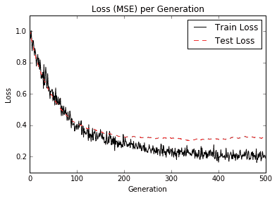我們可以用`matplotlib`和以下代碼繪制損失： ```py plt.plot(loss_vec, 'k-', label='Train Loss') plt.plot(test_loss, 'r--', label='Test Loss') plt.title('Loss (MSE) per Generation') plt.xlabel('Generation') plt.ylabel('Loss') plt.legend(loc='upper right') plt.show() ``` 我們通過繪制下圖來繼續秘籍： ![](https://img.kancloud.cn/e1/5a/e15a8e89257a6650e9a536895a0c4c67_393x281.png) 圖 4：我們繪制了訓練和測試裝置的損失（MSE）。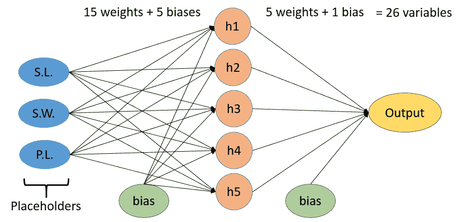請注意，我們在 200 代之后略微過擬合模型，因為測試 MSE 不會進一步下降，但訓練 MSE 確實 ## 工作原理我們的模型現已可視化為神經網絡圖，如下圖所示： ![](https://img.kancloud.cn/c2/e6/c2e658044491f1ecec5d35838399ca73_905x436.png) 圖 5：上圖是我們的神經網絡的可視化，在隱藏層中有五個節點。我們饋送三個值：萼片長度（S.L），萼片寬度（S.W.）和花瓣長度（P.L.）。目標將是花瓣寬度。總的來說，模型中總共有 26 個變量 ## 更多請注意，通過查看測試和訓練集上的`loss`函數，我們可以確定模型何時開始過擬合訓練數據。我們還可以看到訓練損失并不像測試裝置那樣平穩。這是因為有兩個原因：第一個原因是我們使用的批量小于測試集，盡管不是很多；第二個原因是由于我們正在訓練訓練組，而測試裝置不會影響模型的變量。 # 實現不同的層了解如何實現不同的層非常重要。在前面的秘籍中，我們實現了完全連接的層。在本文中，我們將進一步擴展我們對各層的了解。 ## 準備我們已經探索了如何連接數據輸入和完全連接的隱藏層，但是 TensorFlow 中有更多類型的層是內置函數。最常用的層是卷積層和最大池化層。我們將向您展示如何使用輸入數據和完全連接的數據創建和使用此類層。首先，我們將研究如何在一維數據上使用這些層，然后在二維數據上使用這些層。雖然神經網絡可以以任何方式分層，但最常見的用途之一是使用卷積層和完全連接的層來首先創建特征。如果我們有太多的特征，通常會有一個最大池化層。在這些層之后，通常引入非線性層作為激活函數。我們將在第 8 章卷積神經網絡中考慮的卷積神經網絡（CNN）通常具有卷積，最大池化，激活，卷積，最大池化和激活形式。 ## 操作步驟我們將首先看一維數據。我們需要使用以下步驟為此任務生成隨機數據數組： 1. 我們首先加載我們需要的庫并啟動圖會話，如下所示： ```py import tensorflow as tf import numpy as np sess = tf.Session() ``` 1. 現在我們可以初始化我們的數據（長度為`25`的 NumPy 數組）并創建占位符，我們將通過以下代碼提供它： ```py data_size = 25 data_1d = np.random.normal(size=data_size) x_input_1d = tf.placeholder(dtype=tf.float32, shape=[data_size]) ``` 1. 接下來，我們將定義一個將構成卷積層的函數。然后我們將聲明一個隨機過濾器并創建卷積層，如下所示： > 請注意，許多 TensorFlow 的層函數都是為處理 4D 數據而設計的（`4D = [batch size, width, height, and channels]`）。我們需要修改輸入數據和輸出數據，以擴展或折疊所需的額外維度。對于我們的示例數據，我們的批量大小為 1，寬度為 1，高度為 25，通道大小為 1。要擴展大小，我們使用`expand_dims()`函數，并且為了折疊大小，我們使用`squeeze()`函數。另請注意，我們可以使用`output_size=(W-F+2P)/S+1`公式計算卷積層的輸出大小，其中`W`是輸入大小，`F`是濾鏡大小，`P`是填充大小，`S`是步幅大小。 ```py def conv_layer_1d(input_1d, my_filter): # Make 1d input into 4d input_2d = tf.expand_dims(input_1d, 0) input_3d = tf.expand_dims(input_2d, 0) input_4d = tf.expand_dims(input_3d, 3) # Perform convolution convolution_output = tf.nn.conv2d(input_4d, filter=my_filter, strides=[1,1,1,1], padding="VALID") # Now drop extra dimensions conv_output_1d = tf.squeeze(convolution_output) return(conv_output_1d) my_filter = tf.Variable(tf.random_normal(shape=[1,5,1,1])) my_convolution_output = conv_layer_1d(x_input_1d, my_filter) ``` 1. 默認情況下，TensorFlow 的激活函數將按元素方式執行。這意味著我們只需要在感興趣的層上調用激活函數。我們通過創建激活函數然后在圖上初始化它來完成此操作，如下所示： ```py def activation(input_1d): return tf.nn.relu(input_1d) my_activation_output = activation(my_convolution_output) ``` 1. 現在我們將聲明一個最大池化層函數。此函數將在我們的一維向量上的移動窗口上創建一個最大池化。對于此示例，我們將其初始化為寬度為 5，如下所示： > TensorFlow 的最大池化參數與卷積層的參數非常相似。雖然最大池化參數沒有過濾器，但它確實有`size`，`stride`和`padding`選項。由于我們有一個帶有有效填充的 5 的窗口（沒有零填充），因此我們的輸出數組將減少 4 個條目。 ```py def max_pool(input_1d, width): # First we make the 1d input into 4d. input_2d = tf.expand_dims(input_1d, 0) input_3d = tf.expand_dims(input_2d, 0) input_4d = tf.expand_dims(input_3d, 3) # Perform the max pool operation pool_output = tf.nn.max_pool(input_4d, ksize=[1, 1, width, 1], strides=[1, 1, 1, 1], padding='VALID') pool_output_1d = tf.squeeze(pool_output) return pool_output_1d my_maxpool_output = max_pool(my_activation_output, width=5) ``` 1. 我們將要連接的最后一層是完全連接的層。在這里，我們想要創建一個多特征函數，輸入一維數組并輸出指示的數值。還要記住，要使用 1D 數組進行矩陣乘法，我們必須將維度擴展為 2D，如下面的代碼塊所示： ```py def fully_connected(input_layer, num_outputs): # Create weights weight_shape = tf.squeeze(tf.stack([tf.shape(input_layer), [num_outputs]])) weight = tf.random_normal(weight_shape, stddev=0.1) bias = tf.random_normal(shape=[num_outputs]) # Make input into 2d input_layer_2d = tf.expand_dims(input_layer, 0) # Perform fully connected operations full_output = tf.add(tf.matmul(input_layer_2d, weight), bias) # Drop extra dimensions full_output_1d = tf.squeeze(full_output) return full_output_1d my_full_output = fully_connected(my_maxpool_output, 5) ``` 1. 現在我們將初始化所有變量，運行圖并打印每個層的輸出，如下所示： ```py init = tf.global_variable_initializer() sess.run(init) feed_dict = {x_input_1d: data_1d} # Convolution Output print('Input = array of length 25') print('Convolution w/filter, length = 5, stride size = 1, results in an array of length 21:') print(sess.run(my_convolution_output, feed_dict=feed_dict)) # Activation Output print('Input = the above array of length 21') print('ReLU element wise returns the array of length 21:') print(sess.run(my_activation_output, feed_dict=feed_dict)) # Maxpool Output print('Input = the above array of length 21') print('MaxPool, window length = 5, stride size = 1, results in the array of length 17:') print(sess.run(my_maxpool_output, feed_dict=feed_dict)) # Fully Connected Output print('Input = the above array of length 17') print('Fully connected layer on all four rows with five outputs:') print(sess.run(my_full_output, feed_dict=feed_dict)) ``` 1. 上一步應該產生以下輸出： ```py Input = array of length 25 Convolution w/filter, length = 5, stride size = 1, results in an array of length 21: [-0.91608119 1.53731811 -0.7954089 0.5041104 1.88933098 -1.81099761 0.56695032 1.17945457 -0.66252393 -1.90287709 0.87184119 0.84611893 -5.25024986 -0.05473572 2.19293165 -4.47577858 -1.71364677 3.96857905 -2.0452652 -1.86647367 -0.12697852] Input = the above array of length 21 ReLU element wise returns the array of length 21: [ 0\. 1.53731811 0\. 0.5041104 1.88933098 0\. 0\. 1.17945457 0\. 0\. 0.87184119 0.84611893 0\. 0\. 2.19293165 0\. 0\. 3.96857905 0\. 0\. 0\. ] Input = the above array of length 21 MaxPool, window length = 5, stride size = 1, results in the array of length 17: [ 1.88933098 1.88933098 1.88933098 1.88933098 1.88933098 1.17945457 1.17945457 1.17945457 0.87184119 0.87184119 2.19293165 2.19293165 2.19293165 3.96857905 3.96857905 3.96857905 3.96857905] Input = the above array of length 17 Fully connected layer on all four rows with five outputs: [ 1.23588216 -0.42116445 1.44521213 1.40348077 -0.79607368] ``` > 對于神經網絡，一維數據非常重要。時間序列，信號處理和一些文本嵌入被認為是一維的并且經常在神經網絡中使用。我們現在將以相同的順序考慮相同類型的層，但是對于二維數據： 1. 我們將從清除和重置計算圖開始，如下所示： ```py ops.reset_default_graph() sess = tf.Session() ``` 1. 然后我們將初始化我們的輸入數組，使其為`10x10`矩陣，然后我們將為具有相同形狀的圖初始化占位符，如下所示： ```py data_size = [10,10] data_2d = np.random.normal(size=data_size) x_input_2d = tf.placeholder(dtype=tf.float32, shape=data_size) ``` 1. 就像在一維示例中一樣，我們現在需要聲明卷積層函數。由于我們的數據已經具有高度和寬度，我們只需要將其擴展為二維（批量大小為 1，通道大小為 1），以便我們可以使用`conv2d()`函數對其進行操作。對于濾波器，我們將使用隨機`2x2`濾波器，兩個方向的步幅為 2，以及有效填充（換句話說，沒有零填充）。因為我們的輸入矩陣是`10x10`，我們的卷積輸出將是`5x5`，如下所示： ```py def conv_layer_2d(input_2d, my_filter): # First, change 2d input to 4d input_3d = tf.expand_dims(input_2d, 0) input_4d = tf.expand_dims(input_3d, 3) # Perform convolution convolution_output = tf.nn.conv2d(input_4d, filter=my_filter, strides=[1,2,2,1], padding="VALID") # Drop extra dimensions conv_output_2d = tf.squeeze(convolution_output) return(conv_output_2d) my_filter = tf.Variable(tf.random_normal(shape=[2,2,1,1])) my_convolution_output = conv_layer_2d(x_input_2d, my_filter) ``` 1. 激活函數在逐個元素的基礎上工作，因此我們現在可以創建激活操作并使用以下代碼在圖上初始化它： ```py def activation(input_2d): return tf.nn.relu(input_2d) my_activation_output = activation(my_convolution_output) ``` 1. 我們的最大池化層與一維情況非常相似，只是我們必須聲明最大池化窗口的寬度和高度。就像我們的卷積 2D 層一樣，我們只需要擴展到兩個維度，如下所示： ```py def max_pool(input_2d, width, height): # Make 2d input into 4d input_3d = tf.expand_dims(input_2d, 0) input_4d = tf.expand_dims(input_3d, 3) # Perform max pool pool_output = tf.nn.max_pool(input_4d, ksize=[1, height, width, 1], strides=[1, 1, 1, 1], padding='VALID') # Drop extra dimensions pool_output_2d = tf.squeeze(pool_output) return pool_output_2d my_maxpool_output = max_pool(my_activation_output, width=2, height=2) ``` 1. 我們的全連接層與一維輸出非常相似。我們還應該注意到，此層的 2D 輸入被視為一個對象，因此我們希望每個條目都連接到每個輸出。為了實現這一點，我們需要完全展平二維矩陣，然后將其展開以進行矩陣乘法，如下所示： ```py def fully_connected(input_layer, num_outputs): # Flatten into 1d flat_input = tf.reshape(input_layer, [-1]) # Create weights weight_shape = tf.squeeze(tf.stack([tf.shape(flat_input), [num_outputs]])) weight = tf.random_normal(weight_shape, stddev=0.1) bias = tf.random_normal(shape=[num_outputs]) # Change into 2d input_2d = tf.expand_dims(flat_input, 0) # Perform fully connected operations full_output = tf.add(tf.matmul(input_2d, weight), bias) # Drop extra dimensions full_output_2d = tf.squeeze(full_output) return full_output_2d my_full_output = fully_connected(my_maxpool_output, 5) ``` 1. 現在我們需要初始化變量并使用以下代碼為我們的操作創建一個饋送字典： ```py init = tf.global_variables_initializer() sess.run(init) feed_dict = {x_input_2d: data_2d} ``` 1. 每個層的輸出應如下所示： ```py # Convolution Output print('Input = [10 X 10] array') print('2x2 Convolution, stride size = [2x2], results in the [5x5] array:') print(sess.run(my_convolution_output, feed_dict=feed_dict)) # Activation Output print('Input = the above [5x5] array') print('ReLU element wise returns the [5x5] array:') print(sess.run(my_activation_output, feed_dict=feed_dict)) # Max Pool Output print('Input = the above [5x5] array') print('MaxPool, stride size = [1x1], results in the [4x4] array:') print(sess.run(my_maxpool_output, feed_dict=feed_dict)) # Fully Connected Output print('Input = the above [4x4] array') print('Fully connected layer on all four rows with five outputs:') print(sess.run(my_full_output, feed_dict=feed_dict)) ``` 1. 上一步應該產生以下輸出： ```py Input = [10 X 10] array 2x2 Convolution, stride size = [2x2], results in the [5x5] array: [[ 0.37630892 -1.41018617 -2.58821273 -0.32302785 1.18970704] [-4.33685207 1.97415686 1.0844903 -1.18965471 0.84643292] [ 5.23706436 2.46556497 -0.95119286 1.17715418 4.1117816 ] [ 5.86972761 1.2213701 1.59536231 2.66231227 2.28650784] [-0.88964868 -2.75502229 4.3449688 2.67776585 -2.23714781]] Input = the above [5x5] array ReLU element wise returns the [5x5] array: [[ 0.37630892 0\. 0\. 0\. 1.18970704] [ 0\. 1.97415686 1.0844903 0\. 0.84643292] [ 5.23706436 2.46556497 0\. 1.17715418 4.1117816 ] [ 5.86972761 1.2213701 1.59536231 2.66231227 2.28650784] [ 0\. 0\. 4.3449688 2.67776585 0\. ]] Input = the above [5x5] array MaxPool, stride size = [1x1], results in the [4x4] array: [[ 1.97415686 1.97415686 1.0844903 1.18970704] [ 5.23706436 2.46556497 1.17715418 4.1117816 ] [ 5.86972761 2.46556497 2.66231227 4.1117816 ] [ 5.86972761 4.3449688 4.3449688 2.67776585]] Input = the above [4x4] array Fully connected layer on all four rows with five outputs: [-0.6154139 -1.96987963 -1.88811922 0.20010889 0.32519674] ``` ## 工作原理我們現在應該知道如何在 TensorFlow 中使用一維和二維數據中的卷積和最大池化層。無論輸入的形狀如何，我們最終都得到相同的大小輸出。這對于說明神經網絡層的靈活性很重要。本節還應該再次向我們強調形狀和大小在神經網絡操作中的重要性。 # 使用多層神經網絡我們現在將通過在低出生體重數據集上使用多層神經網絡將我們對不同層的知識應用于實際數據。 ## 準備現在我們知道如何創建神經網絡并使用層，我們將應用此方法，以預測低出生體重數據集中的出生體重。我們將創建一個具有三個隱藏層的神經網絡。低出生體重數據集包括實際出生體重和出生體重是否高于或低于 2,500 克的指標變量。在這個例子中，我們將目標設為實際出生體重（回歸），然后在最后查看分類的準確率。最后，我們的模型應該能夠確定出生體重是否小于 2,500 克。 ## 操作步驟我們按如下方式處理秘籍： 1. 我們將首先加載庫并初始化我們的計算圖，如下所示： ```py import tensorflow as tf import matplotlib.pyplot as plt import os import csv import requests import numpy as np sess = tf.Session() ``` 1. 我們現在將使用`requests`模塊從網站加載數據。在此之后，我們將數據拆分為感興趣的特征和目標值，如下所示： ```py # Name of data file birth_weight_file = 'birth_weight.csv' birthdata_url = 'https://github.com/nfmcclure/tensorflow_cookbook/raw/master' \ '/01_Introduction/07_Working_with_Data_Sources/birthweight_data/birthweight.dat' # Download data and create data file if file does not exist in current directory if not os.path.exists(birth_weight_file): birth_file = requests.get(birthdata_url) birth_data = birth_file.text.split('\r\n') birth_header = birth_data[0].split('\t') birth_data = [[float(x) for x in y.split('\t') if len(x) >= 1] for y in birth_data[1:] if len(y) >= 1] with open(birth_weight_file, "w") as f: writer = csv.writer(f) writer.writerows([birth_header]) writer.writerows(birth_data) # Read birth weight data into memory birth_data = [] with open(birth_weight_file, newline='') as csvfile: csv_reader = csv.reader(csvfile) birth_header = next(csv_reader) for row in csv_reader: birth_data.append(row) birth_data = [[float(x) for x in row] for row in birth_data] # Pull out target variable y_vals = np.array([x[0] for x in birth_data]) # Pull out predictor variables (not id, not target, and not birthweight) x_vals = np.array([x[1:8] for x in birth_data]) ``` 1. 為了幫助實現可重復性，我們現在需要為 NumPy 和 TensorFlow 設置隨機種子。然后我們聲明我們的批量大小如下： ```py seed = 4 tf.set_random_seed(seed) np.random.seed(seed) batch_size = 100 ``` 1. 接下來，我們將數據分成 80-20 訓練測試分組。在此之后，我們需要正則化我們的輸入特征，使它們在 0 到 1 之間，具有最小 - 最大縮放比例，如下所示： ```py train_indices = np.random.choice(len(x_vals), round(len(x_vals)*0.8), replace=False) test_indices = np.array(list(set(range(len(x_vals))) - set(train_indices))) x_vals_train = x_vals[train_indices] x_vals_test = x_vals[test_indices] y_vals_train = y_vals[train_indices] y_vals_test = y_vals[test_indices] # Normalize by column (min-max norm) def normalize_cols(m, col_min=np.array([None]), col_max=np.array([None])): if not col_min[0]: col_min = m.min(axis=0) if not col_max[0]: col_max = m.max(axis=0) return (m-col_min) / (col_max - col_min), col_min, col_max x_vals_train, train_min, train_max = np.nan_to_num(normalize_cols(x_vals_train)) x_vals_test, _, _ = np.nan_to_num(normalize_cols(x_vals_test), train_min, train_max) ``` > 歸一化輸入特征是一種常見的特征轉換，尤其適用于神經網絡。如果我們的數據以 0 到 1 的中心為激活函數，它將有助于收斂。 1. 由于我們有多個層具有相似的初始化變量，我們現在需要創建一個函數來初始化權重和偏差。我們使用以下代碼執行此操作： ```py def init_weight(shape, st_dev): weight = tf.Variable(tf.random_normal(shape, stddev=st_dev)) return weight def init_bias(shape, st_dev): bias = tf.Variable(tf.random_normal(shape, stddev=st_dev)) return bias ``` 1. 我們現在需要初始化占位符。將有八個輸入特征和一個輸出，出生重量以克為單位，如下所示： ```py x_data = tf.placeholder(shape=[None, 8], dtype=tf.float32) y_target = tf.placeholder(shape=[None, 1], dtype=tf.float32) ``` 1. 對于所有三個隱藏層，完全連接的層將使用三次。為了防止重復代碼，我們將在初始化模型時創建一個層函數，如下所示： ```py def fully_connected(input_layer, weights, biases): layer = tf.add(tf.matmul(input_layer, weights), biases) return tf.nn.relu(layer) ``` 1. 現在是時候創建我們的模型了。對于每個層（和輸出層），我們將初始化權重矩陣，偏置矩陣和完全連接的層。對于此示例，我們將使用大小為 25，10 和 3 的隱藏層： > 我們使用的模型將有 522 個變量適合。為了得到這個數字，我們可以看到數據和第一個隱藏層之間有`8*25 +25=225`變量。如果我們以這種方式繼續添加它們，我們將有`225+260+33+4=522`變量。這遠遠大于我們在邏輯回歸模型中使用的九個變量。 ```py # Create second layer (25 hidden nodes) weight_1 = init_weight(shape=[8, 25], st_dev=10.0) bias_1 = init_bias(shape=[25], st_dev=10.0) layer_1 = fully_connected(x_data, weight_1, bias_1) # Create second layer (10 hidden nodes) weight_2 = init_weight(shape=[25, 10], st_dev=10.0) bias_2 = init_bias(shape=[10], st_dev=10.0) layer_2 = fully_connected(layer_1, weight_2, bias_2) # Create third layer (3 hidden nodes) weight_3 = init_weight(shape=[10, 3], st_dev=10.0) bias_3 = init_bias(shape=[3], st_dev=10.0) layer_3 = fully_connected(layer_2, weight_3, bias_3) # Create output layer (1 output value) weight_4 = init_weight(shape=[3, 1], st_dev=10.0) bias_4 = init_bias(shape=[1], st_dev=10.0) final_output = fully_connected(layer_3, weight_4, bias_4) ``` 1. 我們現在將使用 L1 損失函數（絕對值），聲明我們的優化器（使用 Adam 優化），并按如下方式初始化變量： ```py loss = tf.reduce_mean(tf.abs(y_target - final_output)) my_opt = tf.train.AdamOptimizer(0.05) train_step = my_opt.minimize(loss) init = tf.global_variables_initializer() sess.run(init) ``` > 雖然我們在前一步驟中用于 Adam 優化函數的學習率是 0.05，但有研究表明較低的學習率始終產生更好的結果。對于這個秘籍，由于數據的一致性和快速收斂的需要，我們使用了更大的學習率。 1. 接下來，我們需要訓練我們的模型進行 200 次迭代。我們還將包含存儲`train`和`test`損失的代碼，選擇隨機批量大小，并每 25 代打印一次狀態，如下所示： ```py # Initialize the loss vectors loss_vec = [] test_loss = [] for i in range(200): # Choose random indices for batch selection rand_index = np.random.choice(len(x_vals_train), size=batch_size) # Get random batch rand_x = x_vals_train[rand_index] rand_y = np.transpose([y_vals_train[rand_index]]) # Run the training step sess.run(train_step, feed_dict={x_data: rand_x, y_target: rand_y}) # Get and store the train loss temp_loss = sess.run(loss, feed_dict={x_data: rand_x, y_target: rand_y}) loss_vec.append(temp_loss) # Get and store the test loss test_temp_loss = sess.run(loss, feed_dict={x_data: x_vals_test, y_target: np.transpose([y_vals_test])}) test_loss.append(test_temp_loss) if (i+1)%25==0: print('Generation: ' + str(i+1) + '. Loss = ' + str(temp_loss)) ``` 1. 上一步應該產生以下輸出： ```py Generation: 25\. Loss = 5922.52 Generation: 50\. Loss = 2861.66 Generation: 75\. Loss = 2342.01 Generation: 100\. Loss = 1880.59 Generation: 125\. Loss = 1394.39 Generation: 150\. Loss = 1062.43 Generation: 175\. Loss = 834.641 Generation: 200\. Loss = 848.54 ``` 1. 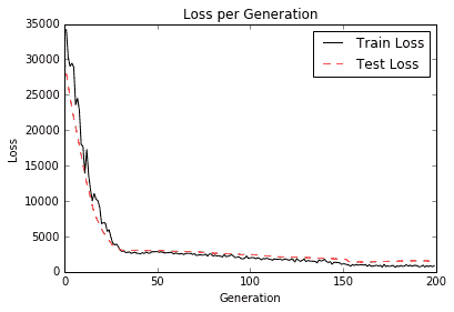以下是使用`matplotlib`繪制訓練和測試損失的代碼片段： ```py plt.plot(loss_vec, 'k-', label='Train Loss') plt.plot(test_loss, 'r--', label='Test Loss') plt.title('Loss per Generation') plt.xlabel('Generation') plt.ylabel('Loss') plt.legend(loc='upper right') plt.show() ``` 我們通過繪制下圖來繼續秘籍： ![](https://img.kancloud.cn/7a/83/7a830e066368db24ac84d6914a67d2a0_409x281.png) 圖 6：在上圖中，我們繪制了我們訓練的神經網絡的訓練和測試損失，以克數表示出生體重。請注意，大約 30 代后我們已經達到了良好的模型 1. 我們現在想將我們的出生體重結果與我們之前的后勤結果進行比較。使用邏輯線性回歸（如第 3 章中的實現邏輯回歸秘籍，線性回歸），我們在數千次迭代后獲得了大約 60% 的準確率結果。為了將其與我們在上一節中所做的進行比較，我們需要輸出訓練并測試回歸結果，并通過創建指標（如果它們高于或低于 2,500 克）將其轉換為分類結果。要找出模型的準確率，我們需要使用以下代碼： ```py actuals = np.array([x[1] for x in birth_data]) test_actuals = actuals[test_indices] train_actuals = actuals[train_indices] test_preds = [x[0] for x in sess.run(final_output, feed_dict={x_data: x_vals_test})] train_preds = [x[0] for x in sess.run(final_output, feed_dict={x_data: x_vals_train})] test_preds = np.array([1.0 if x<2500.0 else 0.0 for x in test_preds]) train_preds = np.array([1.0 if x<2500.0 else 0.0 for x in train_preds]) # Print out accuracies test_acc = np.mean([x==y for x,y in zip(test_preds, test_actuals)]) train_acc = np.mean([x==y for x,y in zip(train_preds, train_actuals)]) print('On predicting the category of low birthweight from regression output (<2500g):') print('Test Accuracy: {}'.format(test_acc)) print('Train Accuracy: {}'.format(train_acc)) ``` 1. 上一步應該產生以下輸出： ```py Test Accuracy: 0.631578947368421 Train Accuracy: 0.7019867549668874 ``` ## 工作原理在這個秘籍中，我們創建了一個回歸神經網絡，其中包含三個完全連接的隱藏層，以預測低出生體重數據集的出生體重。當將其與物流輸出進行比較以預測高于或低于 2,500 克時，我們獲得了類似的結果并且在更少的幾代中實現了它們。在下一個方案中，我們將嘗試通過使其成為多層邏輯類神經網絡來改進邏輯回歸。 # 改進線性模型的預測在前面的秘籍中，我們注意到我們擬合的參數數量遠遠超過等效的線性模型。在這個秘籍中，我們將嘗試通過使用神經網絡來改進我們的低出生體重的邏輯模型。 ## 準備對于這個秘籍，我們將加載低出生體重數據，并使用神經網絡與兩個隱藏的完全連接的層與 sigmoid 激活，以適應低出生體重的概率。 ## 操作步驟我們按如下方式處理秘籍： 1. 我們首先加載庫并初始化我們的計算圖，如下所示： ```py import matplotlib.pyplot as plt import numpy as np import tensorflow as tf import requests sess = tf.Session() ``` 1. 接下來，我們按照前面的秘籍加載，提取和標準化我們的數據，除了在這里我們將使用低出生體重指示變量作為我們的目標而不是實際出生體重，如下所示： ```py # Name of data file birth_weight_file = 'birth_weight.csv' birthdata_url = 'https://github.com/nfmcclure/tensorflow_cookbook/raw/master' \ '/01_Introduction/07_Working_with_Data_Sources/birthweight_data/birthweight.dat' # Download data and create data file if file does not exist in current directory if not os.path.exists(birth_weight_file): birth_file = requests.get(birthdata_url) birth_data = birth_file.text.split('\r\n') birth_header = birth_data[0].split('\t') birth_data = [[float(x) for x in y.split('\t') if len(x) >= 1] for y in birth_data[1:] if len(y) >= 1] with open(birth_weight_file, "w") as f: writer = csv.writer(f) writer.writerows([birth_header]) writer.writerows(birth_data) # read birth weight data into memory birth_data = [] with open(birth_weight_file, newline='') as csvfile: csv_reader = csv.reader(csvfile) birth_header = next(csv_reader) for row in csv_reader: birth_data.append(row) birth_data = [[float(x) for x in row] for row in birth_data] # Pull out target variable y_vals = np.array([x[0] for x in birth_data]) # Pull out predictor variables (not id, not target, and not birthweight) x_vals = np.array([x[1:8] for x in birth_data]) train_indices = np.random.choice(len(x_vals), round(len(x_vals)*0.8), replace=False) test_indices = np.array(list(set(range(len(x_vals))) - set(train_indices))) x_vals_train = x_vals[train_indices] x_vals_test = x_vals[test_indices] y_vals_train = y_vals[train_indices] y_vals_test = y_vals[test_indices] def normalize_cols(m, col_min=np.array([None]), col_max=np.array([None])): if not col_min[0]: col_min = m.min(axis=0) if not col_max[0]: col_max = m.max(axis=0) return (m - col_min) / (col_max - col_min), col_min, col_max x_vals_train, train_min, train_max = np.nan_to_num(normalize_cols(x_vals_train)) x_vals_test, _, _ = np.nan_to_num(normalize_cols(x_vals_test, train_min, train_max)) ``` 1. 接下來，我們需要聲明我們的批量大小和數據的占位符，如下所示： ```py batch_size = 90 x_data = tf.placeholder(shape=[None, 7], dtype=tf.float32) y_target = tf.placeholder(shape=[None, 1], dtype=tf.float32) ``` 1. 如前所述，我們現在需要聲明在模型中初始化變量和層的函數。為了創建更好的邏輯函數，我們需要創建一個在輸入層上返回邏輯層的函數。換句話說，我們將使用完全連接的層并為每個層返回一個 sigmoid 元素。重要的是要記住我們的損失函數將包含最終的 sigmoid，因此我們要在最后一層指定我們不會返回輸出的 sigmoid，如下所示： ```py def init_variable(shape): return tf.Variable(tf.random_normal(shape=shape)) # Create a logistic layer definition def logistic(input_layer, multiplication_weight, bias_weight, activation = True): linear_layer = tf.add(tf.matmul(input_layer, multiplication_weight), bias_weight) if activation: return tf.nn.sigmoid(linear_layer) else: return linear_layer ``` 1. 現在我們將聲明三個層（兩個隱藏層和一個輸出層）。我們將首先為每個層初始化權重和偏差矩陣，并按如下方式定義層操作： ```py # First logistic layer (7 inputs to 14 hidden nodes) A1 = init_variable(shape=[7,14]) b1 = init_variable(shape=[14]) logistic_layer1 = logistic(x_data, A1, b1) # Second logistic layer (14 hidden inputs to 5 hidden nodes) A2 = init_variable(shape=[14,5]) b2 = init_variable(shape=[5]) logistic_layer2 = logistic(logistic_layer1, A2, b2) # Final output layer (5 hidden nodes to 1 output) A3 = init_variable(shape=[5,1]) b3 = init_variable(shape=[1]) final_output = logistic(logistic_layer2, A3, b3, activation=False) ``` 1. 接下來，我們聲明我們的損失（交叉熵）和優化算法，并初始化以下變量： ```py # Create loss function loss = tf.reduce_mean(tf.nn.sigmoid_cross_entropy_with_logits(logits=final_output, labels=y_target)) # Declare optimizer my_opt = tf.train.AdamOptimizer(learning_rate = 0.002) train_step = my_opt.minimize(loss) # Initialize variables init = tf.global_variables_initializer() sess.run(init) ``` > 交叉熵是一種測量概率之間距離的方法。在這里，我們想要測量確定性（0 或 1）與模型概率（`0 < x < 1`）之間的差異。 TensorFlow 使用內置的 sigmoid 函數實現交叉熵。這也是超參數調整的一部分，因為我們更有可能找到最佳的損失函數，學習率和針對當前問題的優化算法。為簡潔起見，我們不包括超參數調整。 1. 為了評估和比較我們的模型與以前的模型，我們需要在圖上創建預測和精度操作。這將允許我們提供整個測試集并確定準確率，如下所示： ```py prediction = tf.round(tf.nn.sigmoid(final_output)) predictions_correct = tf.cast(tf.equal(prediction, y_target), tf.float32) accuracy = tf.reduce_mean(predictions_correct) ``` 1. 我們現在準備開始我們的訓練循環。我們將訓練 1500 代并保存模型損失并訓練和測試精度以便以后進行繪圖。我們的訓練循環使用以下代碼啟動： ```py # Initialize loss and accuracy vectors loss_vec = [] train_acc = [] test_acc = [] for i in range(1500): # Select random indicies for batch selection rand_index = np.random.choice(len(x_vals_train), size=batch_size) # Select batch rand_x = x_vals_train[rand_index] rand_y = np.transpose([y_vals_train[rand_index]]) # Run training step sess.run(train_step, feed_dict={x_data: rand_x, y_target: rand_y}) # Get training loss temp_loss = sess.run(loss, feed_dict={x_data: rand_x, y_target: rand_y}) loss_vec.append(temp_loss) # Get training accuracy temp_acc_train = sess.run(accuracy, feed_dict={x_data: x_vals_train, y_target: np.transpose([y_vals_train])}) train_acc.append(temp_acc_train) # Get test accuracy temp_acc_test = sess.run(accuracy, feed_dict={x_data: x_vals_test, y_target: np.transpose([y_vals_test])}) test_acc.append(temp_acc_test) if (i+1)%150==0: print('Loss = '' + str(temp_loss)) ``` 1. 上一步應該產生以下輸出： ```py Loss = 0.696393 Loss = 0.591708 Loss = 0.59214 Loss = 0.505553 Loss = 0.541974 Loss = 0.512707 Loss = 0.590149 Loss = 0.502641 Loss = 0.518047 Loss = 0.502616 ``` 1. 以下代碼塊說明了如何使用`matplotlib`繪制交叉熵損失以及訓練和測試集精度： ```py # Plot loss over time plt.plot(loss_vec, 'k-') plt.title('Cross Entropy Loss per Generation') plt.xlabel('Generation') plt.ylabel('Cross Entropy Loss') plt.show() # Plot train and test accuracy plt.plot(train_acc, 'k-', label='Train Set Accuracy') plt.plot(test_acc, 'r--', label='Test Set Accuracy') plt.title('Train and Test Accuracy') plt.xlabel('Generation') plt.ylabel('Accuracy') plt.legend(loc='lower right') plt.show() ``` 我們得到每代交叉熵損失的圖如下： ![](https://img.kancloud.cn/7d/16/7d1687642c2bfbb08640b51b6ed1c786_396x281.png) 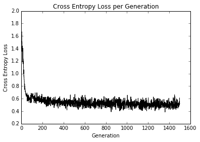圖 7：超過 1500 次迭代的訓練損失在大約 50 代之內，我們已經達到了良好的模式。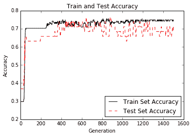在我們繼續訓練時，我們可以看到在剩余的迭代中獲得的很少，如下圖所示： ![](https://img.kancloud.cn/ca/19/ca196ce5b0ef82e14115cdf913277c21_396x281.png) 圖 8：訓練組和測試裝置的準確率正如您在上圖中所看到的，我們很快就找到了一個好模型。 ## 工作原理在考慮使用神經網絡建模數據時，您必須考慮優缺點。雖然我們的模型比以前的模型融合得更快，并且可能具有更高的準確率，但這需要付出代價；我們正在訓練更多的模型變量，并且更有可能過擬合。為了檢查是否發生過擬合，我們會查看測試和訓練集的準確率。如果訓練集的準確率繼續增加而測試集的精度保持不變或甚至略微下降，我們可以假設過擬合正在發生。為了對抗欠擬合，我們可以增加模型深度或訓練模型以進行更多迭代。為了解決過擬合問題，我們可以為模型添加更多數據或添加正則化技術。同樣重要的是要注意我們的模型變量不像線性模型那樣可解釋。神經網絡模型具有比線性模型更難解釋的系數，因為它們解釋了模型中特征的重要性。 # 學習玩井字棋為了展示適應性神經網絡的可用性，我們現在將嘗試使用神經網絡來學習井字棋的最佳動作。我們將知道井字棋是一種確定性游戲，并且最佳動作已經知道。 ## 準備為了訓練我們的模型，我們將使用一系列的棋盤位置，然后對許多不同的棋盤進行最佳的最佳響應。我們可以通過僅考慮在對稱性方面不同的棋盤位置來減少要訓練的棋盤數量。井字棋棋盤的非同一性變換是 90 度，180 度和 270 度的旋轉（在任一方向上），水平反射和垂直反射。鑒于這個想法，我們將使用最佳移動的候選棋盤名單，應用兩個隨機變換，然后將其輸入神經網絡進行學習。 > 由于井字棋是一個確定性的游戲，值得注意的是，無論誰先走，都應該贏或抽。我們希望能夠以最佳方式響應我們的動作并最終獲得平局的模型。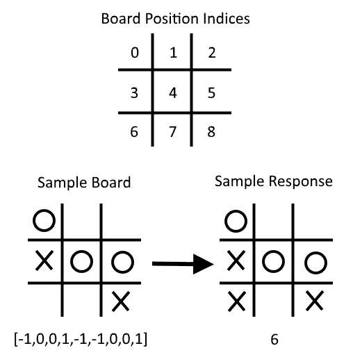如果我們將`X`標注為 1，將`O`標注為 -1，將空格標注為 0，則下圖說明了我們如何將棋盤位置和最佳移動視為一行數據： ![](https://img.kancloud.cn/60/17/6017b1859886ba38034991ca196a7fec_508x524.png)Figure 9: Here, we illustrate how to consider a board and an optimal move as a row of data. Note that X = 1, O = -1, and empty spaces are 0, and we start indexing at 0 除了模型損失，要檢查我們的模型如何執行，我們將做兩件事。我們將執行的第一項檢查是從訓練集中刪除位置和最佳移動行。這將使我們能夠看到神經網絡模型是否可以推廣它以前從未見過的移動。我們將評估模型的第二種方法是在最后實際對抗它。可以在此秘籍的 [GitHub 目錄](https://github.com/nfmcclure/tensorflow_cookbook/tree/master/06_Neural_Networks/08_Learning_Tic_Tac_Toe) 和 [Packt 倉庫](https://github.com/PacktPublishing/TensorFlow-Machine-Learning-Cookbook-Second-Edition)中找到可能的棋盤列表和最佳移動。 ## 操作步驟我們按如下方式處理秘籍： 1. 我們需要從為此腳本加載必要的庫開始，如下所示： ```py import tensorflow as tf import matplotlib.pyplot as plt import csv import random import numpy as np import random ``` 1. 接下來，我們聲明以下批量大小來訓練我們的模型： ```py batch_size = 50 ``` 1. 為了使棋盤更容易可視化，我們將創建一個輸出帶`X`和`O`的井字棋棋盤的函數。這是通過以下代碼完成的： ```py def print_board(board): symbols = ['O', ' ', 'X'] board_plus1 = [int(x) + 1 for x in board] board_line1 = ' {} | {} | {}'.format(symbols[board_plus1[0]], symbols[board_plus1[1]], symbols[board_plus1[2]]) board_line2 = ' {} | {} | {}'.format(symbols[board_plus1[3]], symbols[board_plus1[4]], symbols[board_plus1[5]]) board_line3 = ' {} | {} | {}'.format(symbols[board_plus1[6]], symbols[board_plus1[7]], symbols[board_plus1[8]]) print(board_line1) print('___________') print(board_line2) print('___________') print(board_line3) ``` 1. 現在我們必須創建一個函數，它將返回一個新的棋盤和一個轉換下的最佳響應位置。這是通過以下代碼完成的： ```py def get_symmetry(board, response, transformation): ''' :param board: list of integers 9 long: opposing mark = -1 friendly mark = 1 empty space = 0 :param transformation: one of five transformations on a board: rotate180, rotate90, rotate270, flip_v, flip_h :return: tuple: (new_board, new_response) ''' if transformation == 'rotate180': new_response = 8 - response return board[::-1], new_response elif transformation == 'rotate90': new_response = [6, 3, 0, 7, 4, 1, 8, 5, 2].index(response) tuple_board = list(zip(*[board[6:9], board[3:6], board[0:3]])) return [value for item in tuple_board for value in item], new_response elif transformation == 'rotate270': new_response = [2, 5, 8, 1, 4, 7, 0, 3, 6].index(response) tuple_board = list(zip(*[board[0:3], board[3:6], board[6:9]]))[::-1] return [value for item in tuple_board for value in item], new_response elif transformation == 'flip_v': new_response = [6, 7, 8, 3, 4, 5, 0, 1, 2].index(response) return board[6:9] + board[3:6] + board[0:3], new_response elif transformation == 'flip_h': # flip_h = rotate180, then flip_v new_response = [2, 1, 0, 5, 4, 3, 8, 7, 6].index(response) new_board = board[::-1] return new_board[6:9] + new_board[3:6] + new_board[0:3], new_response else: raise ValueError('Method not implmented.') ``` 1. 棋盤列表及其最佳響應位于目錄中的`.csv`文件中，可從 [github 倉庫](https://github.com/nfmcclure/tensorflow_cookbook)或 [Packt 倉庫](https://github.com/PacktPublishing/TensorFlow-Machine-Learning-Cookbook-Second-Edition)獲得。我們將創建一個函數，它將使用棋盤和響應加載文件，并將其存儲為元組列表，如下所示： ```py def get_moves_from_csv(csv_file): ''' :param csv_file: csv file location containing the boards w/ responses :return: moves: list of moves with index of best response ''' moves = [] with open(csv_file, 'rt') as csvfile: reader = csv.reader(csvfile, delimiter=',') for row in reader: moves.append(([int(x) for x in row[0:9]],int(row[9]))) return moves ``` 1. 現在我們需要將所有內容組合在一起以創建一個函數，該函數將返回隨機轉換的棋盤和響應。這是通過以下代碼完成的： ```py def get_rand_move(moves, rand_transforms=2): # This function performs random transformations on a board. (board, response) = random.choice(moves) possible_transforms = ['rotate90', 'rotate180', 'rotate270', 'flip_v', 'flip_h'] for i in range(rand_transforms): random_transform = random.choice(possible_transforms) (board, response) = get_symmetry(board, response, random_transform) return board, response ``` 1. 接下來，我們需要初始化圖會話，加載數據，并創建一個訓練集，如下所示： ```py sess = tf.Session() moves = get_moves_from_csv('base_tic_tac_toe_moves.csv') # Create a train set: train_length = 500 train_set = [] for t in range(train_length): train_set.append(get_rand_move(moves)) ``` 1. 請記住，我們希望從我們的訓練集中刪除一個棋盤和一個最佳響應，以查看該模型是否可以推廣以實現最佳移動。以下棋盤的最佳舉措將是在第 6 號指數進行： ```py test_board = [-1, 0, 0, 1, -1, -1, 0, 0, 1] train_set = [x for x in train_set if x[0] != test_board] ``` 1. 我們現在可以創建函數來創建模型變量和模型操作。請注意，我們在以下模型中不包含`softmax()`激活函數，因為它包含在損失函數中： ```py def init_weights(shape): return tf.Variable(tf.random_normal(shape)) def model(X, A1, A2, bias1, bias2): layer1 = tf.nn.sigmoid(tf.add(tf.matmul(X, A1), bias1)) layer2 = tf.add(tf.matmul(layer1, A2), bias2) return layer2 ``` 1. 現在我們需要聲明我們的占位符，變量和模型，如下所示： ```py X = tf.placeholder(dtype=tf.float32, shape=[None, 9]) Y = tf.placeholder(dtype=tf.int32, shape=[None]) A1 = init_weights([9, 81]) bias1 = init_weights([81]) A2 = init_weights([81, 9]) bias2 = init_weights([9]) model_output = model(X, A1, A2, bias1, bias2) ``` 1. 接下來，我們需要聲明我們的`loss`函數，它將是最終輸出對率的平均 softmax（非標準化輸出）。然后我們將聲明我們的訓練步驟和優化器。如果我們希望將來能夠對抗我們的模型，我們還需要創建一個預測操作，如下所示： ```py loss = tf.reduce_mean(tf.nn.sparse_softmax_cross_entropy_with_logits(logits=model_output, labels=Y)) train_step = tf.train.GradientDescentOptimizer(0.025).minimize(loss) prediction = tf.argmax(model_output, 1) ``` 1. 我們現在可以使用以下代碼初始化變量并循環遍歷神經網絡的訓練： ```py # Initialize variables init = tf.global_variables_initializer() sess.run(init) loss_vec = [] for i in range(10000): # Select random indices for batch rand_indices = np.random.choice(range(len(train_set)), batch_size, replace=False) # Get batch batch_data = [train_set[i] for i in rand_indices] x_input = [x[0] for x in batch_data] y_target = np.array([y[1] for y in batch_data]) # Run training step sess.run(train_step, feed_dict={X: x_input, Y: y_target}) # Get training loss temp_loss = sess.run(loss, feed_dict={X: x_input, Y: y_target}) loss_vec.append(temp_loss) ``` ```py if i%500==0: print('iteration ' + str(i) + ' Loss: ' + str(temp_loss)) ``` 1. 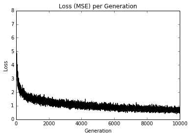以下是繪制模型訓練損失所需的代碼： ```py plt.plot(loss_vec, 'k-', label='Loss') plt.title('Loss (MSE) per Generation') plt.xlabel('Generation') plt.ylabel('Loss') plt.show() ``` 我們應該得到以下每代損失的繪圖： ![](https://img.kancloud.cn/08/27/082703a41ea92ae20a9b7a114ccc0a5f_390x281.png) 圖 10：超過 10,000 次迭代的井字棋訓練組損失在上圖中，我們繪制了訓練步驟的損失。 1. 為了測試模型，我們需要看看它是如何在我們從訓練集中刪除的測試棋盤上執行的。我們希望模型可以推廣和預測移動的最佳索引，這將是索引號 6。大多數時候模型將成功，如下所示： ```py test_boards = [test_board] feed_dict = {X: test_boards} logits = sess.run(model_output, feed_dict=feed_dict) predictions = sess.run(prediction, feed_dict=feed_dict) print(predictions) ``` 1. 上一步應該產生以下輸出： ```py [6] ``` 1. 為了評估我們的模型，我們需要與我們訓練的模型進行對比。要做到這一點，我們必須創建一個能夠檢查勝利的函數。這樣，我們的程序將知道何時停止要求更多動作。這是通過以下代碼完成的： ```py def check(board): wins = [[0,1,2], [3,4,5], [6,7,8], [0,3,6], [1,4,7], [2,5,8], [0,4,8], [2,4,6]] for i in range(len(wins)): if board[wins[i][0]]==board[wins[i][1]]==board[wins[i][2]]==1.: return 1 elif board[wins[i][0]]==board[wins[i][1]]==board[wins[i][2]]==-1.: return 1 return 0 ``` 1. 現在我們可以使用我們的模型循環播放游戲。我們從一個空白棋盤（全零）開始，我們要求用戶輸入一個索引（0-8），然后我們將其輸入到模型中進行預測。對于模型的移動，我們采用最大的可用預測，也是一個開放空間。從這個游戲中，我們可以看到我們的模型并不完美，如下所示： ```py game_tracker = [0., 0., 0., 0., 0., 0., 0., 0., 0.] win_logical = False num_moves = 0 while not win_logical: player_index = input('Input index of your move (0-8): ') num_moves += 1 # Add player move to game game_tracker[int(player_index)] = 1\. # Get model's move by first getting all the logits for each index [potential_moves] = sess.run(model_output, feed_dict={X: [game_tracker]}) # Now find allowed moves (where game tracker values = 0.0) allowed_moves = [ix for ix,x in enumerate(game_tracker) if x==0.0] # Find best move by taking argmax of logits if they are in allowed moves model_move = np.argmax([x if ix in allowed_moves else -999.0 for ix,x in enumerate(potential_moves)]) # Add model move to game game_tracker[int(model_move)] = -1\. print('Model has moved') print_board(game_tracker) # Now check for win or too many moves if check(game_tracker)==1 or num_moves>=5: print('Game Over!') win_logical = True ``` 1. 上一步應該產生以下交互輸出： ```py Input index of your move (0-8): 4 Model has moved O | | ___________ | X | ___________ | | Input index of your move (0-8): 6 Model has moved O | | ___________ | X | ___________ X | | O Input index of your move (0-8): 2 Model has moved O | | X ___________ O | X | ___________ X | | O Game Over! ``` ## 工作原理在本節中，我們通過饋送棋盤位置和九維向量訓練神經網絡來玩井字棋，并預測最佳響應。我們只需要喂幾個可能的井字棋棋盤并對每個棋盤應用隨機變換以增加訓練集大小。為了測試我們的算法，我們刪除了一個特定棋盤的所有實例，并查看我們的模型是否可以推廣以預測最佳響應。最后，我們針對我們的模型玩了一個示例游戲。雖然它還不完善，但仍有不同的架構和訓練程序可用于改進它。