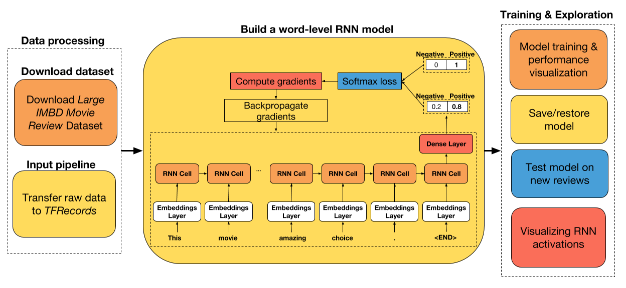
# 八、用于 TensorFlow Eager 序列分類的動態循壞神經網絡 大家好！ 在本教程中，我們將構建一個循環神經網絡，用于對 IMDB 電影評論進行情感分析。 我選擇了這個數據集，因為它很小，很容易被任何人下載，所以數據采集沒有瓶頸。 本教程的主要目的不是教你如何構建一個簡單的 RNN，而是如何構建一個 RNN，為你提供模型開發的更大靈活性（例如，使用目前在 Keras 中不可用的新 RNN 單元，更容易訪問 RNN 的展開輸出，從磁盤批量讀取數據）。 我希望能夠讓你看看，在你可能感興趣的任何領域中，如何繼續建立你自己的模型，不管它們有多復雜。 教程步驟  + 下載原始數據并將其轉換為 TFRecords（ TensorFlow 默認文件格式）。 + 準備一個數據集迭代器，它從磁盤中批量讀取數據，并自動將可變長度的輸入數據填充到批量中的最大大小。 + 使用 LSTM 和 UGRNN 單元構建單詞級 RNN 模型。 + 在測試數據集上比較兩個單元的性能。 + 保存/恢復訓練模型 + 在新評論上測試網絡 + 可視化 RNN 激活 如果你想在本教程中添加任何內容，請告訴我們。 此外，我很高興聽到你的任何改進建議。 ## 導入實用的庫 ```py # 導入函數來編寫和解析 TFRecords from data_utils import imdb2tfrecords from data_utils import parse_imdb_sequence # 導入 TensorFlow 和 TensorFlow Eager import tensorflow as tf import tensorflow.contrib.eager as tfe # 為數據處理導入 pandas，為數據讀取導入 pickle import pandas as pd import pickle # 導入繪圖庫 import matplotlib.pyplot as plt %matplotlib inline # 開啟 Eager 模式。一旦開啟不能撤銷！只執行一次。 tfe.enable_eager_execution(device_policy=tfe.DEVICE_PLACEMENT_SILENT) ``` ## 下載數據并轉換為 TFRecords 或者，如果你克隆這個倉庫，你將自動將下載的數據解析為 TFRecords，因此請隨意跳過此步驟。 大型電影評論數據集是“二元情感分類的數據集，包含比以前的基準數據集更多的數據”（來源）。 它由 25000 個評論的訓練數據集（12500 個正面和 125000 個負面）和 25000 個評論的測試數據集（12500 個正面和 125000 個負面）組成。 以下是正面評論的示例： > Rented the movie as a joke. My friends and I had so much fun laughing at it that I went and found a used copy and bought it for myself. Now when all my friends are looking for a funny movie I give them Sasquatch Hunters. It needs to be said though there is a rule that was made that made the movie that much better. No talking is allowed while the movie is on unless the words are Sasquatch repeated in a chant. I loved the credit at the end of the movie as well. "Thanks for the Jeep, Tom!" Whoever Tom is I say thank you because without your Jeep the movie may not have been made. In short a great movie if you are looking for something to laugh at. If you want a good movie maybe look for something else but if you don't mind a laugh at the expense of a man in a monkey suit grab yourself a copy. 以下是負面評論的示例： > The Good: I liked this movie because it was the first horror movie I've seen in a long time that actually scared me. The acting wasn't too bad, and the "Cupid" killer was believable and disturbing. The Bad: The story line and plot of this movie is incredibly weak. There just wasn't much to it. The ways the killer killed his victims was very horrifying and disgusting. I do not recommend this movie to anyone who can not handle gore. Overall: A good scare, but a bad story. 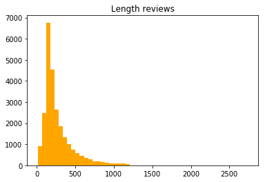為了下載數據集，只需在終端中執行： ``` chmod o+x datasets/get_imdb_dataset.sh datasets/get_imdb_dataset.sh ``` 讓我們來看看評論長度的分布（單詞/評論）： ```py length_reviews = pickle.load(open('datasets/aclImdb/length_reviews.pkl', 'rb')) pd.DataFrame(length_reviews, columns=['Length reviews']).hist(bins=50, color='orange'); plt.grid(False); ```  似乎大多數評論都有大約 250 個單詞。 然而，由于一些相當長的評論，分布似乎有一個很長的尾巴。 由于我們必須將可變長度輸入序列填充到批量中的最大序列，因此保留這些評論將是非常低效的。 因此，我在`imdb2tfrecords`函數中添加了一個參數，你可以在其中指定評論中允許的最大字數。 這將簡單地采用評論中的最后一個`max_words`來提高訓練效率，并避免在很多時間步長內展開神經網絡，這可能導致內存問題。 下載數據集后，只需運行`imdb2tfrecords`函數即可。 此函數將每個評論解析為單詞索引列表。 ```py # 用于將原始數據轉換為 TFRecords 的函數，將評論中每個單詞轉換為整數索引 #imdb2tfrecords(path_data='datasets/aclImdb/', min_word_frequency=5, max_words_review=700) ``` 處理結束時，每個`tfrecord`將由以下內容組成： | TFrecord | 描述 | | --- | --- | | 'token_indexes' | 評論中出現的單詞索引的序列 | | 'target' | 負面情感為 0，正面情感為 1 | | 'sequence_length' | 評論的序列長度 | 如果你想使用新數據集測試此 RNN 網絡，請查看`data_utils.py`腳本中的`imdb2tfrecords`或`parse_imdb_sequence`，來了解如何將新數據解析為 TFRecords。 我真的建議使用這種文件格式，因為它非常容易處理非常大的數據集，而不受 RAM 容量的限制。 ## 創建訓練和測試迭代器 ```py train_dataset = tf.data.TFRecordDataset('datasets/aclImdb/train.tfrecords') train_dataset = train_dataset.map(parse_imdb_sequence).shuffle(buffer_size=10000) train_dataset = train_dataset.padded_batch(512, padded_shapes=([None],[],[])) test_dataset = tf.data.TFRecordDataset('datasets/aclImdb/test.tfrecords') test_dataset = test_dataset.map(parse_imdb_sequence).shuffle(buffer_size=10000) test_dataset = test_dataset.padded_batch(512, padded_shapes=([None],[],[])) # 讀取詞匯表 word2idx = pickle.load(open('datasets/aclImdb/word2idx.pkl', 'rb')) ``` ## 用于序列分類的 RNN 模型，兼容 Eager API 在下面的單元格中，你可以找到我為 RNN 模型創建的類。 API 與我在上一個教程中創建的 API 非常相似，只是現在我們跟蹤模型的準確率而不是損失。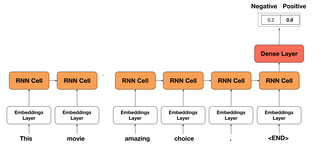 網絡的想法非常簡單。 我們只需在評論中選擇每個單詞，選擇相應的單詞嵌入（在開頭隨機初始化），然后將其傳遞給 RNN 單元。 然后，我們在序列的末尾獲取 RNN 單元的輸出并將其傳遞通過密集層（具有 ReL U激活）來獲得最終預測。 通常，網絡繼承自`tf.keras.Model`，以便跟蹤所有變量并輕松保存/恢復它們。  ```py class RNNModel(tf.keras.Model): def __init__(self, embedding_size=100, cell_size=64, dense_size=128, num_classes=2, vocabulary_size=None, rnn_cell='lstm', device='cpu:0', checkpoint_directory=None): ''' 定義在正向傳播期間使用的參數化層，你要在其上運行計算的設備，以及檢查點目錄。另外，你還可以修改網絡的默認大小。 Args: embedding_size: the size of the word embedding. cell_size: RNN cell size. dense_size: the size of the dense layer. num_classes: the number of labels in the network. vocabulary_size: the size of the word vocabulary. rnn_cell: string, either 'lstm' or 'ugrnn'. device: string, 'cpu:n' or 'gpu:n' (n can vary). Default, 'cpu:0'. checkpoint_directory: the directory where you would like to save or restore a model. ''' super(RNNModel, self).__init__() # 權重初始化函數 w_initializer = tf.contrib.layers.xavier_initializer() # 偏置初始化函數 b_initializer = tf.zeros_initializer() # 為單詞嵌入初始化權重 self.embeddings = tf.keras.layers.Embedding(vocabulary_size, embedding_size, embeddings_initializer=w_initializer) # 密集層的初始化 self.dense_layer = tf.keras.layers.Dense(dense_size, activation=tf.nn.relu, kernel_initializer=w_initializer, bias_initializer=b_initializer) # 預測層的初始化 self.pred_layer = tf.keras.layers.Dense(num_classes, activation=None, kernel_initializer=w_initializer, bias_initializer=b_initializer) # 基本的 LSTM 單元 if rnn_cell=='lstm': self.rnn_cell = tf.nn.rnn_cell.BasicLSTMCell(cell_size) # 否則是 UGRNN 單元 else: self.rnn_cell = tf.contrib.rnn.UGRNNCell(cell_size) # 定義設備 self.device = device # 定義檢查點目錄 self.checkpoint_directory = checkpoint_directory def predict(self, X, seq_length, is_training): ''' 基于輸入樣本，預測每個類的概率 Args: X: 2D tensor of shape (batch_size, time_steps). seq_length: the length of each sequence in the batch. is_training: Boolean. Either the network is predicting in training mode or not. ''' # 獲取批量中的樣本量 num_samples = tf.shape(X)[0] # 初始化 LSTM 單元狀態為零 state = self.rnn_cell.zero_state(num_samples, dtype=tf.float32) # 獲取序列中每個詞的嵌入 embedded_words = self.embeddings(X) # 分割嵌入 unstacked_embeddings = tf.unstack(embedded_words, axis=1) # 遍歷每個時間步長并附加預測 outputs = [] for input_step in unstacked_embeddings: output, state = self.rnn_cell(input_step, state) outputs.append(output) # 將輸出堆疊為（批量大小，時間步長，單元數） outputs = tf.stack(outputs, axis=1) # 對于每個樣本，提取最后一個時間步驟的輸出 idxs_last_output = tf.stack([tf.range(num_samples), tf.cast(seq_length-1, tf.int32)], axis=1) final_output = tf.gather_nd(outputs, idxs_last_output) # 為正則化添加 dropout dropped_output = tf.layers.dropout(final_output, rate=0.3, training=is_training) # 向密集層（ReLU 激活）傳入最后單元的狀態 dense = self.dense_layer(dropped_output) # 計算非標準化的對數概率 logits = self.pred_layer(dense) return logits def loss_fn(self, X, y, seq_length, is_training): """ 定義訓練期間使用的損失函數 """ preds = self.predict(X, seq_length, is_training) loss = tf.losses.sparse_softmax_cross_entropy(labels=y, logits=preds) return loss def grads_fn(self, X, y, seq_length, is_training): """ 在每個正向步驟中， 動態計算損失值對模型參數的梯度 """ with tfe.GradientTape() as tape: loss = self.loss_fn(X, y, seq_length, is_training) return tape.gradient(loss, self.variables) def restore_model(self): """ 用于恢復訓練模型的函數 """ with tf.device(self.device): # 運行模型一次來初始變量 dummy_input = tf.constant(tf.zeros((1,1))) dummy_length = tf.constant(1, shape=(1,)) dummy_pred = self.predict(dummy_input, dummy_length, False) # 恢復模型變量 saver = tfe.Saver(self.variables) saver.restore(tf.train.latest_checkpoint (self.checkpoint_directory)) def save_model(self, global_step=0): """ 用于保存訓練模型的函數 """ tfe.Saver(self.variables).save(self.checkpoint_directory, global_step=global_step) def fit(self, training_data, eval_data, optimizer, num_epochs=500, early_stopping_rounds=10, verbose=10, train_from_scratch=False): """ 用于訓練模型的函數， 使用所選的優化器，執行所需數量的迭代 你可以從零開始訓練，或者加載最后訓練的模型 使用了提前停止來降低網絡的過擬合風險 Args: training_data: the data you would like to train the model on. Must be in the tf.data.Dataset format. eval_data: the data you would like to evaluate the model on. Must be in the tf.data.Dataset format. optimizer: the optimizer used during training. num_epochs: the maximum number of iterations you would like to train the model. early_stopping_rounds: stop training if the accuracy on the eval dataset does not increase after n epochs. verbose: int. Specify how often to print the loss value of the network. train_from_scratch: boolean. Whether to initialize variables of the the last trained model or initialize them randomly. """ if train_from_scratch==False: self.restore_model() # 初始化 best_acc。這個變量儲存最高的準確率。 # on the eval dataset. best_acc = 0 # 初始化類別來更新訓練和評估的平均準確率 train_acc = tfe.metrics.Accuracy('train_acc') eval_acc = tfe.metrics.Accuracy('eval_acc') # 初始化字典來存儲準確率歷史 self.history = {} self.history['train_acc'] = [] self.history['eval_acc'] = [] # 開始訓練 with tf.device(self.device): for i in range(num_epochs): # 使用梯度下降來訓練 for X, y, seq_length in tfe.Iterator(training_data): grads = self.grads_fn(X, y, seq_length, True) optimizer.apply_gradients(zip(grads, self.variables)) # 檢查訓練集的準確率 for X, y, seq_length in tfe.Iterator(training_data): logits = self.predict(X, seq_length, False) preds = tf.argmax(logits, axis=1) train_acc(preds, y) self.history['train_acc'].append(train_acc.result().numpy()) # 重置指標 train_acc.init_variables() # 檢查評估集的準確率 for X, y, seq_length in tfe.Iterator(eval_data): logits = self.predict(X, seq_length, False) preds = tf.argmax(logits, axis=1) eval_acc(preds, y) self.history['eval_acc'].append(eval_acc.result().numpy()) # 重置指標 eval_acc.init_variables() # 打印訓練和評估準確率 if (i==0) | ((i+1)%verbose==0): print('Train accuracy at epoch %d: ' %(i+1), self.history['train_acc'][-1]) print('Eval accuracy at epoch %d: ' %(i+1), self.history['eval_acc'][-1]) # 為提前停止而檢查 if self.history['eval_acc'][-1]>best_acc: best_acc = self.history['eval_acc'][-1] count = early_stopping_rounds else: count -= 1 if count==0: break ``` ## 使用梯度下降和提前停止來訓練模型 ### 使用簡單的 LSTM 單元來訓練模型 ```py # 指定你打算存儲/恢復訓練變量的路徑 checkpoint_directory = 'models_checkpoints/ImdbRNN/' # 如果可用，則使用 GPU device = 'gpu:0' if tfe.num_gpus()>0 else 'cpu:0' # 定義優化器 optimizer = tf.train.AdamOptimizer(learning_rate=1e-4) # 初始化模型，還沒有初始化變量 lstm_model = RNNModel(vocabulary_size=len(word2idx), device=device, checkpoint_directory=checkpoint_directory) # 訓練模型 lstm_model.fit(train_dataset, test_dataset, optimizer, num_epochs=500, early_stopping_rounds=5, verbose=1, train_from_scratch=True) ''' Train accuracy at epoch 1: 0.72308 Eval accuracy at epoch 1: 0.68372 Train accuracy at epoch 2: 0.77708 Eval accuracy at epoch 2: 0.75472 Train accuracy at epoch 3: 0.875 Eval accuracy at epoch 3: 0.82036 Train accuracy at epoch 4: 0.91728 Eval accuracy at epoch 4: 0.8542 Train accuracy at epoch 5: 0.94728 Eval accuracy at epoch 5: 0.87464 Train accuracy at epoch 6: 0.96312 Eval accuracy at epoch 6: 0.88228 Train accuracy at epoch 7: 0.97476 Eval accuracy at epoch 7: 0.88624 Train accuracy at epoch 8: 0.9828 Eval accuracy at epoch 8: 0.88344 Train accuracy at epoch 9: 0.98692 Eval accuracy at epoch 9: 0.87036 Train accuracy at epoch 10: 0.99052 Eval accuracy at epoch 10: 0.86724 Train accuracy at epoch 11: 0.9944 Eval accuracy at epoch 11: 0.87088 Train accuracy at epoch 12: 0.99568 Eval accuracy at epoch 12: 0.86068 ''' # 保存模型 lstm_model.save_model() ``` ### 使用 UGRNN 單元訓練模型 ```py # 定義優化器 optimizer = tf.train.AdamOptimizer(learning_rate=1e-4) # 初始化模型，還沒有初始化變量 ugrnn_model = RNNModel(vocabulary_size=len(word2idx), rnn_cell='ugrnn', device=device, checkpoint_directory=checkpoint_directory) # 訓練模型 ugrnn_model.fit(train_dataset, test_dataset, optimizer, num_epochs=500, early_stopping_rounds=5, verbose=1, train_from_scratch=True) ''' Train accuracy at epoch 1: 0.71092 Eval accuracy at epoch 1: 0.67688 Train accuracy at epoch 2: 0.82512 Eval accuracy at epoch 2: 0.7982 Train accuracy at epoch 3: 0.88792 Eval accuracy at epoch 3: 0.84116 Train accuracy at epoch 4: 0.92156 Eval accuracy at epoch 4: 0.85076 Train accuracy at epoch 5: 0.94592 Eval accuracy at epoch 5: 0.86476 Train accuracy at epoch 6: 0.95984 Eval accuracy at epoch 6: 0.87104 Train accuracy at epoch 7: 0.9708 Eval accuracy at epoch 7: 0.87188 Train accuracy at epoch 8: 0.9786 Eval accuracy at epoch 8: 0.8748 Train accuracy at epoch 9: 0.98412 Eval accuracy at epoch 9: 0.86452 Train accuracy at epoch 10: 0.9882 Eval accuracy at epoch 10: 0.86172 Train accuracy at epoch 11: 0.9938 Eval accuracy at epoch 11: 0.86808 Train accuracy at epoch 12: 0.9956 Eval accuracy at epoch 12: 0.8596 Train accuracy at epoch 13: 0.997 Eval accuracy at epoch 13: 0.86368 ''' ``` ### 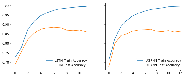表現比較 ```py f, (ax1, ax2) = plt.subplots(1, 2, sharey=True, figsize=(10, 4)) ax1.plot(range(len(lstm_model.history['train_acc'])), lstm_model.history['train_acc'], label='LSTM Train Accuracy'); ax1.plot(range(len(lstm_model.history['eval_acc'])), lstm_model.history['eval_acc'], label='LSTM Test Accuracy'); ax2.plot(range(len(ugrnn_model.history['train_acc'])), ugrnn_model.history['train_acc'], label='UGRNN Train Accuracy'); ax2.plot(range(len(ugrnn_model.history['eval_acc'])), ugrnn_model.history['eval_acc'], label='UGRNN Test Accuracy'); ax1.legend(); ax2.legend(); ```  ## 在新評論上測試網絡 我認為最近在 IMDb 上發布的新評論測試網絡會很不錯。 我選擇了 2018 年 2 月為電影 Bad Apples 發布的三條評論。 隨意試試新的評論或自己發布一個新的評論！ 網絡能在所有三種情況下正確識別情感，所以我印象非常深刻。 ```py ################################################################ # 恢復訓練模型 ################################################################ tf.reset_default_graph() checkpoint_directory = 'models_checkpoints/ImdbRNN/' device = 'gpu:0' if tfe.num_gpus()>0 else 'cpu:0' lstm_model = RNNModel(vocabulary_size=len(word2idx), device=device, checkpoint_directory=checkpoint_directory) lstm_model.restore_model() # INFO:tensorflow:Restoring parameters from models_checkpoints/ImdbRNN/-0 ############################################################### # 導入/下載必要的庫來處理新的序列 ############################################################### import nltk try: nltk.data.find('tokenizers/punkt') except LookupError: nltk.download('punkt') from nltk.tokenize import word_tokenize import re def process_new_review(review): '''用于處理新評論的函數 Args: review: original text review, string. Returns: indexed_review: sequence of integers, words correspondence from word2idx. seq_length: the length of the review. ''' indexed_review = re.sub(r'<[^>]+>', ' ', review) indexed_review = word_tokenize(indexed_review) indexed_review = [word2idx[word] if word in list(word2idx.keys()) else word2idx['Unknown_token'] for word in indexed_review] indexed_review = indexed_review + [word2idx['End_token']] seq_length = len(indexed_review) return indexed_review, seq_length sent_dict = {0: 'negative', 1: 'positive'} review_score_10 = "I think Bad Apples is a great time and I recommend! I enjoyed the opening, which gave way for the rest of the movie to occur. The main couple was very likable and I believed all of their interactions. They had great onscreen chemistry and made me laugh quite a few times! Keeping the girls in the masks but seeing them in action was something I loved. It kept a mystery to them throughout. I think the dialogue was great. The kills were fun. And the special surprise gore effect at the end was AWESOME!! I won't spoil that part ;) I also enjoyed how the movie wrapped up. It gave a very urban legends type feel of \"did you ever hear the story...\". Plus is leaves the door open for another film which I wouldn't mind at all. Long story short, I think if you take the film for what it is; a fun little horror flick, then you won't be disappointed! HaPpY eArLy HaLLoWeEn!" review_score_4 = "A young couple comes to a small town, where the husband get a job working in a hospital. The wife which you instantly hate or dislike works home, at the same time a horrible murders takes place in this small town by two masked killers. Bad Apples is just your tipical B-horror movie with average acting (I give them that. Altough you may get the idea that some of the actors are crazy-convervative Christians), but the script is just bad, and that's what destroys the film." review_score_1 = "When you first start watching this movie, you can tell its going to be a painful ride. the audio is poor...the attacks by the \"girls\" are like going back in time, to watching the old rocky films, were blows never touched. the editing is poor with it aswell, example the actress in is the bath when her husband comes home, clearly you see her wearing a flesh coloured bra in the bath. no hints or spoilers, just wait till you find it in a bargain basket of cheap dvds in a couple of weeks" new_reviews = [review_score_10, review_score_4, review_score_1] scores = [10, 4, 1] with tf.device(device): for original_review, score in zip(new_reviews, scores): indexed_review, seq_length = process_new_review(original_review) indexed_review = tf.reshape(tf.constant(indexed_review), (1,-1)) seq_length = tf.reshape(tf.constant(seq_length), (1,)) logits = lstm_model.predict(indexed_review, seq_length, False) pred = tf.argmax(logits, axis=1).numpy()[0] print('The sentiment for the review with score %d was found to be %s' %(score, sent_dict[pred])) ''' The sentiment for the review with score 10 was found to be positive The sentiment for the review with score 4 was found to be negative The sentiment for the review with score 1 was found to be negative ''' ``` ## 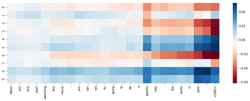展示 RNN 單元的激活 本教程的部分內容受到了 Karpathy 在[《可視化和理解循壞神經網絡》](https://arxiv.org/abs/1506.02078)中的工作的啟發。 我們將使用`seaborn`庫繪制熱圖。 你可以通過在終端輸入這個來獲取它： ``` pip install seaborn ``` ```py # 導入用于 RNN 可視化的庫 import seaborn as sns def VisualizeRNN(model, X): ''' 返回每個時間步驟的單元狀態的 tanh 的函數 Args: model: trained RNN model. X: indexed review of shape (1, sequence_length). Returns: tanh(cell_states): the tanh of the memory cell at each timestep. ''' # 初始化 LSTM 單元狀態為零 state = model.rnn_cell.zero_state(1, dtype=tf.float32) # 獲取序列中每個詞的嵌入 embedded_words = model.embeddings(X) # 分割嵌入 unstacked_embeddings = tf.unstack(embedded_words, axis=1) # 遍歷每個時間步驟，附加它的單元狀態 cell_states = [] for input_step in unstacked_embeddings: _, state = model.rnn_cell(input_step, state) cell_states.append(state[0]) # 將 cell_states 堆疊為（批量大小，時間步長，單元數量） cell_states = tf.stack(cell_states, axis=1) return tf.tanh(cell_states) # 隨意修改輸入 dummy_review = "When you first start watching this movie, you can tell its going to be a painful ride. the audio is poor..." # 處理新的評論 indexed_review, seq_length = process_new_review(dummy_review) indexed_review = tf.reshape(tf.constant(indexed_review), (1,-1)) # 獲取單元狀態 cell_states = VisualizeRNN(lstm_model, indexed_review) # 繪制單元中前 10 個單元的激活（總共有 64 個單元） plt.figure(figsize = (16,5)) sns.heatmap(cell_states.numpy()[0,:,:10].T, xticklabels=word_tokenize(dummy_review)+['<END>'], cmap='RdBu'); ```