# 八、卷積神經網絡 卷積神經網絡（CNN）負責過去幾年中圖像識別的重大突破。在本章中，我們將介紹以下主題： * 實現簡單的 CNN * 實現高級的 CNN * 重新訓練現有的 CNN 模型 * 應用 Stylenet 和神經式項目 * 實現 DeepDream > 提醒一下，讀者可以在[這里](https://github.com/nfmcclure/tensorflow_cookbook)，以及 [Packt 倉庫](https://github.com/PacktPublishing/TensorFlow-Machine-Learning-Cookbook-Second-Edition)找到本章的所有代碼。 # 介紹 在數學中，卷積是應用于另一個函數的輸出的函數。在我們的例子中，我們將考慮在圖像上應用矩陣乘法（濾波器）。出于我們的目的，我們將圖像視為數字矩陣。這些數字可以表示像素或甚至圖像屬性。我們將應用于這些矩陣的卷積運算包括在圖像上移動固定寬度的濾波器并應用逐元素乘法來得到我們的結果。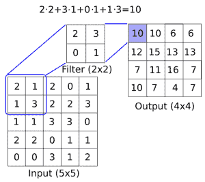 有關圖像卷積如何工作的概念性理解，請參見下圖：  圖 1：如何在圖像上應用卷積濾鏡（長度與寬度之間的深度），以創建新的特征層。這里，我們有一個`2x2`卷積濾波器，在`5x5`輸入的有效空間中操作，兩個方向的步幅為 1。結果是`4x4`矩陣 CNN 還具有滿足更多要求的其他操作，例如引入非線性（ReLU）或聚合參數（最大池化）以及其他類似操作。上圖是在`5x5`數組上應用卷積運算的示例，其中卷積濾波器是`2x2`矩陣。步長為 1，我們只考慮有效的展示位置。此操作中的可訓練變量將是`2x2`濾波器權重。在卷積之后，通常會跟進聚合操作，例如最大池化。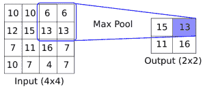如果我們在兩個方向上采用步幅為 2 的`2x2`區域的最大值，下圖提供了最大池如何操作的示例：  圖 2：最大池化操作如何運行的示例。這里，我們有一個`2x2`窗口，在`4x4`輸入的有效空間上操作，兩個方向的步幅為 2。結果是`2x2`矩陣 雖然我們將首先創建自己的 CNN 進行圖像識別，但強烈建議您使用現有的架構，我們將在本章的其余部分中進行操作。 > 通常采用預先訓練好的網絡并使用新數據集對其進行重新訓練，并在最后使用新的完全連接層。這種方法非常有用，我們將在重新訓練現有的 CNN 模型秘籍中進行說明，我們將重新訓練現有的架構以改進我們的 CIFAR-10 預測。 # 實現簡單的 CNN 在本文中，我們將開發一個四層卷積神經網絡，以提高我們預測 MNIST 數字的準確率。前兩個卷積層將各自由卷積-ReLU-最大池化操作組成，最后兩個層將是完全連接的層。 ## 準備 為了訪問 MNIST 數據，TensorFlow 有一個`examples.tutorials`包，它具有很好的數據集加載函數。加載數據后，我們將設置模型變量，創建模型，批量訓練模型，然后可視化損失，準確率和一些樣本數字。 ## 操作步驟 執行以下步驟： 1. 首先，我們將加載必要的庫并啟動圖會話： ```py import matplotlib.pyplot as plt import numpy as np import tensorflow as tf from tensorflow.examples.tutorials.mnist import input_data from tensorflow.python.framework import ops ops.reset_default_graph() sess = tf.Session() ``` 1. 接下來，我們將加載數據并將圖像轉換為`28x28`數組： ```py data_dir = 'temp' mnist = input_data.read_data_sets(data_dir, one_hot=False) train_xdata = np.array([np.reshape(x, (28,28)) for x in mnist.train.images]) test_xdata = np.array([np.reshape(x, (28,28)) for x in mnist.test.images]) train_labels = mnist.train.labels test_labels = mnist.test.labels ``` > 請注意，此處下載的 MNIST 數據集還包括驗證集。此驗證集通常與測試集的大小相同。如果我們進行任何超參數調整或模型選擇，最好將其加載到其他測試中。 1. 現在我們將設置模型參數。請記住，圖像的深度（通道數）為 1，因為這些圖像是灰度的： ```py batch_size = 100 learning_rate = 0.005 evaluation_size = 500 image_width = train_xdata[0].shape[0] image_height = train_xdata[0].shape[1] target_size = max(train_labels) + 1 num_channels = 1 generations = 500 eval_every = 5 conv1_features = 25 conv2_features = 50 max_pool_size1 = 2 max_pool_size2 = 2 fully_connected_size1 = 100 ``` 1. 我們現在可以聲明數據的占位符。我們將聲明我們的訓練數據變量和測試數據變量。我們將針對訓練和評估規模使用不同的批量大小。您可以根據可用于訓練和評估的物理內存來更改這些內容： ```py x_input_shape = (batch_size, image_width, image_height, num_channels) x_input = tf.placeholder(tf.float32, shape=x_input_shape) y_target = tf.placeholder(tf.int32, shape=(batch_size)) eval_input_shape = (evaluation_size, image_width, image_height, num_channels) eval_input = tf.placeholder(tf.float32, shape=eval_input_shape) eval_target = tf.placeholder(tf.int32, shape=(evaluation_size)) ``` 1. 我們將使用我們在前面步驟中設置的參數聲明我們的卷積權重和偏差： ```py conv1_weight = tf.Variable(tf.truncated_normal([4, 4, num_channels, conv1_features], stddev=0.1, dtype=tf.float32)) conv1_bias = tf.Variable(tf.zeros([conv1_features],dtype=tf.float32)) conv2_weight = tf.Variable(tf.truncated_normal([4, 4, conv1_features, conv2_features], stddev=0.1, dtype=tf.float32)) conv2_bias = tf.Variable(tf.zeros([conv2_features],dtype=tf.float32)) ``` 1. 接下來，我們將為模型的最后兩層聲明完全連接的權重和偏差： ```py resulting_width = image_width // (max_pool_size1 * max_pool_size2) resulting_height = image_height // (max_pool_size1 * max_pool_size2) full1_input_size = resulting_width * resulting_height*conv2_features full1_weight = tf.Variable(tf.truncated_normal([full1_input_size, fully_connected_size1], stddev=0.1, dtype=tf.float32)) full1_bias = tf.Variable(tf.truncated_normal([fully_connected_size1], stddev=0.1, dtype=tf.float32)) full2_weight = tf.Variable(tf.truncated_normal([fully_connected_size1, target_size], stddev=0.1, dtype=tf.float32)) full2_bias = tf.Variable(tf.truncated_normal([target_size], stddev=0.1, dtype=tf.float32)) ``` 1. 現在我們將宣布我們的模型。我們首先創建一個模型函數。請注意，該函數將在全局范圍內查找所需的層權重和偏差。此外，為了使完全連接的層工作，我們將第二個卷積層的輸出展平，這樣我們就可以在完全連接的層中使用它： ```py def my_conv_net(input_data): # First Conv-ReLU-MaxPool Layer conv1 = tf.nn.conv2d(input_data, conv1_weight, strides=[1, 1, 1, 1], padding='SAME') relu1 = tf.nn.relu(tf.nn.bias_add(conv1, conv1_bias)) max_pool1 = tf.nn.max_pool(relu1, ksize=[1, max_pool_size1, max_pool_size1, 1], strides=[1, max_pool_size1, max_pool_size1, 1], padding='SAME') # Second Conv-ReLU-MaxPool Layer conv2 = tf.nn.conv2d(max_pool1, conv2_weight, strides=[1, 1, 1, 1], padding='SAME') relu2 = tf.nn.relu(tf.nn.bias_add(conv2, conv2_bias)) max_pool2 = tf.nn.max_pool(relu2, ksize=[1, max_pool_size2, max_pool_size2, 1], strides=[1, max_pool_size2, max_pool_size2, 1], padding='SAME') # Transform Output into a 1xN layer for next fully connected layer final_conv_shape = max_pool2.get_shape().as_list() final_shape = final_conv_shape[1] * final_conv_shape[2] * final_conv_shape[3] flat_output = tf.reshape(max_pool2, [final_conv_shape[0], final_shape]) # First Fully Connected Layer fully_connected1 = tf.nn.relu(tf.add(tf.matmul(flat_output, full1_weight), full1_bias)) # Second Fully Connected Layer final_model_output = tf.add(tf.matmul(fully_connected1, full2_weight), full2_bias) return final_model_output ``` 1. 接下來，我們可以在訓練和測試數據上聲明模型： ```py model_output = my_conv_net(x_input) test_model_output = my_conv_net(eval_input) ``` 1. 我們將使用的損失函數是 softmax 函數。我們使用稀疏 softmax，因為我們的預測只是一個類別，而不是多個類別。我們還將使用一個對對率而不是縮放概率進行操作的損失函數： ```py loss = tf.reduce_mean(tf.nn.sparse_softmax_cross_entropy_with_logits(logits=model_output, labels=y_target)) ``` 1. 接下來，我們將創建一個訓練和測試預測函數。然后我們還將創建一個準確率函數來確定模型在每個批次上的準確率： ```py prediction = tf.nn.softmax(model_output) test_prediction = tf.nn.softmax(test_model_output) # Create accuracy function def get_accuracy(logits, targets): batch_predictions = np.argmax(logits, axis=1) num_correct = np.sum(np.equal(batch_predictions, targets)) return 100\. * num_correct/batch_predictions.shape[0] ``` 1. 現在我們將創建我們的優化函數，聲明訓練步驟，并初始化所有模型變量： ```py my_optimizer = tf.train.MomentumOptimizer(learning_rate, 0.9) train_step = my_optimizer.minimize(loss) # Initialize Variables init = tf.global_variables_initializer() sess.run(init) ``` 1. 我們現在可以開始訓練我們的模型。我們以隨機選擇的批次循環數據。我們經常選擇在訓練上評估模型并測試批次并記錄準確率和損失。我們可以看到，經過 500 代，我們可以在測試數據上快速達到 96%-97% 的準確率： ```py train_loss = [] train_acc = [] test_acc = [] for i in range(generations): rand_index = np.random.choice(len(train_xdata), size=batch_size) rand_x = train_xdata[rand_index] rand_x = np.expand_dims(rand_x, 3) rand_y = train_labels[rand_index] train_dict = {x_input: rand_x, y_target: rand_y} sess.run(train_step, feed_dict=train_dict) temp_train_loss, temp_train_preds = sess.run([loss, prediction], feed_dict=train_dict) temp_train_acc = get_accuracy(temp_train_preds, rand_y) if (i+1) % eval_every == 0: eval_index = np.random.choice(len(test_xdata), size=evaluation_size) eval_x = test_xdata[eval_index] eval_x = np.expand_dims(eval_x, 3) eval_y = test_labels[eval_index] test_dict = {eval_input: eval_x, eval_target: eval_y} test_preds = sess.run(test_prediction, feed_dict=test_dict) temp_test_acc = get_accuracy(test_preds, eval_y) # Record and print results train_loss.append(temp_train_loss) train_acc.append(temp_train_acc) test_acc.append(temp_test_acc) acc_and_loss = [(i+1), temp_train_loss, temp_train_acc, temp_test_acc] acc_and_loss = [np.round(x,2) for x in acc_and_loss] print('Generation # {}. Train Loss: {:.2f}. Train Acc (Test Acc): {:.2f} ({:.2f})'.format(*acc_and_loss)) ``` 1. 這產生以下輸出： ```py Generation # 5\. Train Loss: 2.37\. Train Acc (Test Acc): 7.00 (9.80) Generation # 10\. Train Loss: 2.16\. Train Acc (Test Acc): 31.00 (22.00) Generation # 15\. Train Loss: 2.11\. Train Acc (Test Acc): 36.00 (35.20) ... Generation # 490\. Train Loss: 0.06\. Train Acc (Test Acc): 98.00 (97.40) Generation # 495\. Train Loss: 0.10\. Train Acc (Test Acc): 98.00 (95.40) Generation # 500\. Train Loss: 0.14\. Train Acc (Test Acc): 98.00 (96.00) ``` 1. 以下是使用`Matplotlib`繪制損耗和精度的代碼： ```py eval_indices = range(0, generations, eval_every) # Plot loss over time plt.plot(eval_indices, train_loss, 'k-') plt.title('Softmax Loss per Generation') plt.xlabel('Generation') plt.ylabel('Softmax Loss') plt.show() # Plot train and test accuracy plt.plot(eval_indices, train_acc, 'k-', label='Train Set Accuracy') plt.plot(eval_indices, test_acc, 'r--', label='Test Set Accuracy') plt.title('Train and Test Accuracy') plt.xlabel('Generation') plt.ylabel('Accuracy') plt.legend(loc='lower right') plt.show() ``` 然后我們得到以下圖：  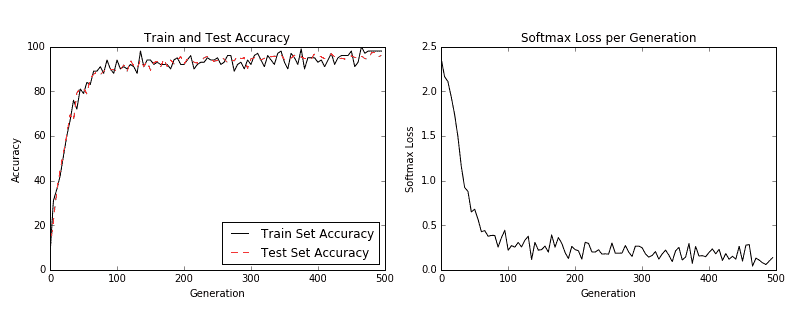圖 3：左圖是我們 500 代訓練中的訓練和測試集精度。右圖是超過 500 代的 softmax 損失值。 1. 如果我們想要繪制最新批次結果的樣本，下面是繪制由六個最新結果組成的樣本的代碼： ```py # Plot the 6 of the last batch results: actuals = rand_y[0:6] predictions = np.argmax(temp_train_preds,axis=1)[0:6] images = np.squeeze(rand_x[0:6]) Nrows = 2 Ncols = 3 for i in range(6): plt.subplot(Nrows, Ncols, i+1) plt.imshow(np.reshape(images[i], [28,28]), cmap='Greys_r') plt.title('Actual: ' + str(actuals[i]) + ' Pred: ' + str(predictions[i]), fontsize=10) frame = plt.gca() frame.axes.get_xaxis().set_visible(False) frame.axes.get_yaxis().set_visible(False) ``` 我們得到前面代碼的以下輸出：  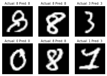圖 4：六個隨機圖像的繪圖，標題中包含實際值和預測值。右下圖預計是 3，而事實上它是 1 ## 工作原理 我們提高了 MNIST 數據集的表現，并構建了一個模型，在從頭開始訓練時，可快速達到約 97% 的準確率。我們的前兩層是卷積，ReLU 和最大池化的組合。第二層是完全連接的層。我們以 100 個批次進行了訓練，并研究了我們訓練的幾代的準確率和損失。最后，我們還繪制了六個隨機數字和每個數字的預測/實際值。 CNN 非常適合圖像識別。造成這種情況的部分原因是卷積層創建了自己的低級特征，當它們遇到重要的部分圖像時會被激活。這種類型的模型自己創建特征并將其用于預測。 ## 更多 在過去幾年中，CNN 模型在圖像識別方面取得了巨大進步。正在探索許多新穎的想法，并且經常發現新的架構。該領域的一個很好的論文庫是一個名為 [Arxiv.org](https://arxiv.org/) 的倉庫網站，由康奈爾大學創建和維護。 Arxiv.org 包括許多領域的一些最新論文，包括計算機科學和計算機科學子領域，如[計算機視覺和圖像識別](https://arxiv.org/list/cs.CV/recent)。 ## 另見 以下列出了一些可用于了解 CNN 的優秀資源： * [斯坦福大學有一個很棒的維基](http://scarlet.stanford.edu/teach/index.php/An_Introduction_to_Convolutional_Neural_Networks) * [邁克爾·尼爾森的深度學習](http://neuralnetworksanddeeplearning.com/chap6.html) * [吳建新介紹卷積神經網絡](https://pdfs.semanticscholar.org/450c/a19932fcef1ca6d0442cbf52fec38fb9d1e5.pdf) # 實現高級的 CNN 能夠擴展 CNN 模型以進行圖像識別非常重要，這樣我們才能理解如何增加網絡的深度。如果我們有足夠的數據，這可能會提高我們預測的準確率。擴展 CNN 網絡的深度是以標準方式完成的：我們只是重復卷積，最大池和 ReLU，直到我們對深度感到滿意為止。許多更精確的圖像識別網絡以這種方式操作。 ## 準備 在本文中，我們將實現一種更先進的讀取圖像數據的方法，并使用更大的 CNN 在 [CIFAR10](https://www.cs.toronto.edu/~kriz/cifar.html) 數據集上進行圖像識別。該數據集具有 60,000 個`32x32`圖像，這些圖像恰好屬于十個可能類別中的一個。圖像的潛在類別是飛機，汽車，鳥，貓，鹿，狗，青蛙，馬，船和卡車。另見“另見”部分中的第一個要點。 大多數圖像數據集太大而無法放入內存中。我們可以使用 TensorFlow 設置一個圖像管道，一次從一個文件中一次讀取。我們通過設置圖像閱讀器，然后創建在圖像閱讀器上運行的批量隊列來完成此操作。 此外，對于圖像識別數據，通常在將圖像發送之前隨機擾動圖像以進行訓練。在這里，我們將隨機裁剪，翻轉和更改亮度。 此秘籍是TensorFlow CIFAR-10 官方教程的改編版本，可在本章末尾的“另見”部分中找到。我們將教程濃縮為一個腳本，我們將逐行完成并解釋所有必要的代碼。我們還將一些常量和參數恢復為原始引用的紙張值；我們將在適當的步驟中標記這一點。 ## 操作步驟 執行以下步驟： 1. 首先，我們加載必要的庫并啟動圖會話： ```py import os import sys import tarfile import matplotlib.pyplot as plt import numpy as np import tensorflow as tf from six.moves import urllib sess = tf.Session() ``` 1. 現在我們將聲明一些模型參數。我們的批量大小為 128（用于訓練和測試）。我們將每 50 代輸出一次狀態，總共運行 20,000 代。每 500 代，我們將評估一批測試數據。然后我們將聲明一些圖像參數，高度和寬度，以及隨機裁剪圖像的大小。有三個通道（紅色，綠色和藍色），我們有十個不同的目標。然后我們將聲明我們將從隊列中存儲數據和圖像批次的位置： ```py batch_size = 128 output_every = 50 generations = 20000 eval_every = 500 image_height = 32 image_width = 32 crop_height = 24 crop_width = 24 num_channels = 3 num_targets = 10 data_dir = 'temp' extract_folder = 'cifar-10-batches-bin' ``` 1. 建議您在我們向好的模型邁進時降低學習率，因此我們將以指數方式降低學習率：初始學習率將設置為 0.1，并且我們將以 250% 的指數方式將其降低 10% 代。確切的公式將由`0.1 · 0.9^(x / 250)`給出，其中`x`是當前世代號。默認情況下，此值會持續降低，但 TensorFlow 會接受僅更新學習率的階梯參數。這里我們設置一些參數供將來使用： ```py learning_rate = 0.1 lr_decay = 0.9 num_gens_to_wait = 250\. ``` 1. 現在我們將設置參數，以便我們可以讀取二進制 CIFAR-10 圖像： ```py image_vec_length = image_height * image_width * num_channels record_length = 1 + image_vec_length ``` 1. 接下來，我們將設置數據目錄和 URL 以下載 CIFAR-10 圖像，如果我們還沒有它們： ```py data_dir = 'temp' if not os.path.exists(data_dir): os.makedirs(data_dir) cifar10_url = 'http://www.cs.toronto.edu/~kriz/cifar-10-binary.tar.gz' data_file = os.path.join(data_dir, 'cifar-10-binary.tar.gz') if not os.path.isfile(data_file): # Download file filepath, _ = urllib.request.urlretrieve(cifar10_url, data_file) # Extract file tarfile.open(filepath, 'r:gz').extractall(data_dir) ``` 1. 我們將設置記錄閱讀器并使用以下`read_cifar_files()`函數返回隨機失真的圖像。首先，我們需要聲明一個讀取固定字節長度的記錄讀取器對象。在我們讀取圖像隊列之后，我們將圖像和標簽分開。最后，我們將使用 TensorFlow 的內置圖像修改函數隨機扭曲圖像： ```py def read_cifar_files(filename_queue, distort_images = True): reader = tf.FixedLengthRecordReader(record_bytes=record_length) key, record_string = reader.read(filename_queue) record_bytes = tf.decode_raw(record_string, tf.uint8) # Extract label image_label = tf.cast(tf.slice(record_bytes, [0], [1]), tf.int32) # Extract image image_extracted = tf.reshape(tf.slice(record_bytes, [1], [image_vec_length]), [num_channels, image_height, image_width]) # Reshape image image_uint8image = tf.transpose(image_extracted, [1, 2, 0]) reshaped_image = tf.cast(image_uint8image, tf.float32) # Randomly Crop image final_image = tf.image.resize_image_with_crop_or_pad(reshaped_image, crop_width, crop_height) if distort_images: # Randomly flip the image horizontally, change the brightness and contrast final_image = tf.image.random_flip_left_right(final_image) final_image = tf.image.random_brightness(final_image,max_delta=63) final_image = tf.image.random_contrast(final_image,lower=0.2, upper=1.8) # Normalize whitening final_image = tf.image.per_image_standardization(final_image) return final_image, image_label ``` 1. 現在我們將聲明一個函數，它將填充我們的圖像管道以供批量器使用。我們首先需要設置一個我們想要讀取的圖像文件列表，并定義如何使用通過預構建的 TensorFlow 函數創建的輸入生成器對象來讀取它們。輸入生成器可以傳遞給我們在上一步中創建的讀取函數：`read_cifar_files()`。然后我們將在隊列中設置批量閱讀器：`shuffle_batch()`： ```py def input_pipeline(batch_size, train_logical=True): if train_logical: files = [os.path.join(data_dir, extract_folder, 'data_batch_{}.bin'.format(i)) for i in range(1,6)] else: files = [os.path.join(data_dir, extract_folder, 'test_batch.bin')] filename_queue = tf.train.string_input_producer(files) image, label = read_cifar_files(filename_queue) min_after_dequeue = 1000 capacity = min_after_dequeue + 3 * batch_size example_batch, label_batch = tf.train.shuffle_batch([image, label], batch_size, capacity, min_after_dequeue) return example_batch, label_batch ``` > 正確設置`min_after_dequeue`很重要。此參數負責設置用于采樣的圖像緩沖區的最小大小。TensorFlow 官方文檔建議將其設置為`(#threads + error margin)*batch_size`。請注意，將其設置為更大的大小會導致更均勻的混洗，因為它正在從隊列中的更大數據集進行混洗，但是在此過程中也將使用更多內存。 1. 接下來，我們可以聲明我們的模型函數。我們將使用的模型有兩個卷積層，后面是三個完全連接的層。為了使變量聲明更容易，我們首先聲明兩個變量函數。兩個卷積層將分別創建 64 個特征。第一個完全連接的層將第二個卷積層與 384 個隱藏節點連接起來。第二個完全連接的操作將這 384 個隱藏節點連接到 192 個隱藏節點。最后的隱藏層操作將 192 個節點連接到我們試圖預測的 10 個輸出類。請參閱以下`#`前面的內聯注釋： ```py def cifar_cnn_model(input_images, batch_size, train_logical=True): def truncated_normal_var(name, shape, dtype): return tf.get_variable(name=name, shape=shape, dtype=dtype, initializer=tf.truncated_normal_initializer(stddev=0.05)) def zero_var(name, shape, dtype): return tf.get_variable(name=name, shape=shape, dtype=dtype, initializer=tf.constant_initializer(0.0)) # First Convolutional Layer with tf.variable_scope('conv1') as scope: # Conv_kernel is 5x5 for all 3 colors and we will create 64 features conv1_kernel = truncated_normal_var(name='conv_kernel1', shape=[5, 5, 3, 64], dtype=tf.float32) # We convolve across the image with a stride size of 1 conv1 = tf.nn.conv2d(input_images, conv1_kernel, [1, 1, 1, 1], padding='SAME') # Initialize and add the bias term conv1_bias = zero_var(name='conv_bias1', shape=[64], dtype=tf.float32) conv1_add_bias = tf.nn.bias_add(conv1, conv1_bias) # ReLU element wise relu_conv1 = tf.nn.relu(conv1_add_bias) # Max Pooling pool1 = tf.nn.max_pool(relu_conv1, ksize=[1, 3, 3, 1], strides=[1, 2, 2, 1],padding='SAME', name='pool_layer1') # Local Response Normalization norm1 = tf.nn.lrn(pool1, depth_radius=5, bias=2.0, alpha=1e-3, beta=0.75, name='norm1') # Second Convolutional Layer with tf.variable_scope('conv2') as scope: # Conv kernel is 5x5, across all prior 64 features and we create 64 more features conv2_kernel = truncated_normal_var(name='conv_kernel2', shape=[5, 5, 64, 64], dtype=tf.float32) # Convolve filter across prior output with stride size of 1 conv2 = tf.nn.conv2d(norm1, conv2_kernel, [1, 1, 1, 1], padding='SAME') # Initialize and add the bias conv2_bias = zero_var(name='conv_bias2', shape=[64], dtype=tf.float32) conv2_add_bias = tf.nn.bias_add(conv2, conv2_bias) # ReLU element wise relu_conv2 = tf.nn.relu(conv2_add_bias) # Max Pooling pool2 = tf.nn.max_pool(relu_conv2, ksize=[1, 3, 3, 1], strides=[1, 2, 2, 1], padding='SAME', name='pool_layer2') # Local Response Normalization (parameters from paper) norm2 = tf.nn.lrn(pool2, depth_radius=5, bias=2.0, alpha=1e-3, beta=0.75, name='norm2') # Reshape output into a single matrix for multiplication for the fully connected layers reshaped_output = tf.reshape(norm2, [batch_size, -1]) reshaped_dim = reshaped_output.get_shape()[1].value # First Fully Connected Layer with tf.variable_scope('full1') as scope: # Fully connected layer will have 384 outputs. full_weight1 = truncated_normal_var(name='full_mult1', shape=[reshaped_dim, 384], dtype=tf.float32) full_bias1 = zero_var(name='full_bias1', shape=[384], dtype=tf.float32) full_layer1 = tf.nn.relu(tf.add(tf.matmul(reshaped_output, full_weight1), full_bias1)) # Second Fully Connected Layer with tf.variable_scope('full2') as scope: # Second fully connected layer has 192 outputs. full_weight2 = truncated_normal_var(name='full_mult2', shape=[384, 192], dtype=tf.float32) full_bias2 = zero_var(name='full_bias2', shape=[192], dtype=tf.float32) full_layer2 = tf.nn.relu(tf.add(tf.matmul(full_layer1, full_weight2), full_bias2)) # Final Fully Connected Layer -> 10 categories for output (num_targets) with tf.variable_scope('full3') as scope: # Final fully connected layer has 10 (num_targets) outputs. full_weight3 = truncated_normal_var(name='full_mult3', shape=[192, num_targets], dtype=tf.float32) full_bias3 = zero_var(name='full_bias3', shape=[num_targets], dtype=tf.float32) final_output = tf.add(tf.matmul(full_layer2, full_weight3), full_bias3) return final_output ``` > 我們的本地響應標準化參數取自本文，并在本文的“另見”部分中引用。 1. 現在我們將創建損失函數。我們將使用 softmax 函數，因為圖片只能占用一個類別，因此輸出應該是十個目標的概率分布： ```py def cifar_loss(logits, targets): # Get rid of extra dimensions and cast targets into integers targets = tf.squeeze(tf.cast(targets, tf.int32)) # Calculate cross entropy from logits and targets cross_entropy = tf.nn.sparse_softmax_cross_entropy_with_logits(logits=logits, labels=targets) # Take the average loss across batch size cross_entropy_mean = tf.reduce_mean(cross_entropy) return cross_entropy_mean ``` 1. 接下來，我們宣布我們的訓練步驟。學習率將以指數階躍函數降低： ```py def train_step(loss_value, generation_num): # Our learning rate is an exponential decay (stepped down) model_learning_rate = tf.train.exponential_decay(learning_rate, generation_num, num_gens_to_wait, lr_decay, staircase=True) # Create optimizer my_optimizer = tf.train.GradientDescentOptimizer(model_learning_rate) # Initialize train step train_step = my_optimizer.minimize(loss_value) return train_step ``` 1. 我們還必須具有精確度函數，以計算一批圖像的準確率。我們將輸入對率目標向量，并輸出平均精度。然后我們可以將它用于訓練和測試批次： ```py def accuracy_of_batch(logits, targets): # Make sure targets are integers and drop extra dimensions targets = tf.squeeze(tf.cast(targets, tf.int32)) # Get predicted values by finding which logit is the greatest batch_predictions = tf.cast(tf.argmax(logits, 1), tf.int32) # Check if they are equal across the batch predicted_correctly = tf.equal(batch_predictions, targets) # Average the 1's and 0's (True's and False's) across the batch size accuracy = tf.reduce_mean(tf.cast(predicted_correctly, tf.float32)) return accuracy ``` 1. 現在我們有了一個圖像管道函數，我們可以初始化訓練圖像管道和測試圖像管道： ```py images, targets = input_pipeline(batch_size, train_logical=True) test_images, test_targets = input_pipeline(batch_size, train_logical=False) ``` 1. 接下來，我們將初始化訓練輸出和測試輸出的模型。值得注意的是，我們必須在創建訓練模型后聲明`scope.reuse_variables()`，這樣，當我們為測試網絡聲明模型時，它將使用相同的模型參數： ```py with tf.variable_scope('model_definition') as scope: # Declare the training network model model_output = cifar_cnn_model(images, batch_size) # Use same variables within scope scope.reuse_variables() # Declare test model output test_output = cifar_cnn_model(test_images, batch_size) ``` 1. 我們現在可以初始化我們的損耗和測試精度函數。然后我們將聲明`generation`變量。此變量需要聲明為不可訓練，并傳遞給我們的訓練函數，該函數在學習率指數衰減計算中使用它： ```py loss = cifar_loss(model_output, targets) accuracy = accuracy_of_batch(test_output, test_targets) generation_num = tf.Variable(0, trainable=False) train_op = train_step(loss, generation_num) ``` 1. 我們現在將初始化所有模型的變量，然后通過運行 TensorFlow 函數`start_queue_runners()`來啟動圖像管道。當我們開始訓練或測試模型輸出時，管道將輸入一批圖像來代替飼料字典： ```py init = tf.global_variables_initializer() sess.run(init) tf.train.start_queue_runners(sess=sess) ``` 1. 我們現在循環訓練我們的訓練，節省訓練損失和測試準確率： ```py train_loss = [] test_accuracy = [] for i in range(generations): _, loss_value = sess.run([train_op, loss]) if (i+1) % output_every == 0: train_loss.append(loss_value) output = 'Generation {}: Loss = {:.5f}'.format((i+1), loss_value) print(output) if (i+1) % eval_every == 0: [temp_accuracy] = sess.run([accuracy]) test_accuracy.append(temp_accuracy) acc_output = ' --- Test Accuracy= {:.2f}%.'.format(100\. * temp_accuracy) print(acc_output) ``` 1. 這產生以下輸出： ```py ... Generation 19500: Loss = 0.04461 --- Test Accuracy = 80.47%. Generation 19550: Loss = 0.01171 Generation 19600: Loss = 0.06911 Generation 19650: Loss = 0.08629 Generation 19700: Loss = 0.05296 Generation 19750: Loss = 0.03462 Generation 19800: Loss = 0.03182 Generation 19850: Loss = 0.07092 Generation 19900: Loss = 0.11342 Generation 19950: Loss = 0.08751 Generation 20000: Loss = 0.02228 --- Test Accuracy = 83.59%. ``` 1. 最后，這里有一些`matplotlib`代碼將繪制在訓練過程中的損失和測試準確率： ```py eval_indices = range(0, generations, eval_every) output_indices = range(0, generations, output_every) # Plot loss over time plt.plot(output_indices, train_loss, 'k-') plt.title('Softmax Loss per Generation') plt.xlabel('Generation') plt.ylabel('Softmax Loss') plt.show() # Plot accuracy over time plt.plot(eval_indices, test_accuracy, 'k-') plt.title('Test Accuracy') plt.xlabel('Generation') plt.ylabel('Accuracy') plt.show() ``` 我們得到以下秘籍的以下繪圖：  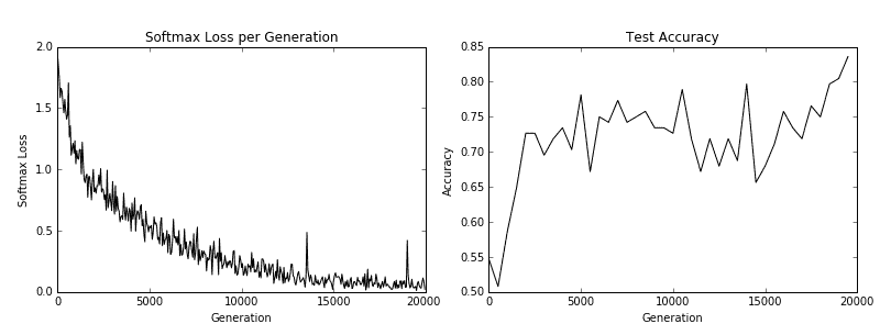圖 5：訓練損失在左側，測試精度在右側。對于 CIFAR-10 圖像識別 CNN，我們能夠實現在測試集上達到約 75% 準確率的模型 ## 工作原理 在我們下載了 CIFAR-10 數據之后，我們建立了一個圖像管道而不是使用源字典。有關圖像管道的更多信息，請參閱 TensorFlow CIFAR-10 官方教程。我們使用此訓練和測試管道來嘗試預測圖像的正確類別。最后，該模型在測試集上達到了約 75% 的準確率。 ## 另見 * 有關 CIFAR-10 數據集的更多信息，[請參閱學習 Tiny Images 的多個特征層，Alex Krizhevsky，2009](https://www.cs.toronto.edu/~kriz/learning-features-2009-TR.pdf) * 要查看原始的 TensorFlow 代碼，請參閱[此鏈接](https://github.com/tensorflow/models/tree/master/tutorials/image/cifar10) * 有關局部響應歸一化的更多信息，請參閱[使用深度卷積神經網絡的 ImageNet 分類，Krizhevsky，A. 等人，2012](http://papers.nips.cc/paper/4824-imagenet-classification-with-deep-convolutional-neural-networks) # 重新訓練現有的 CNN 模型 從頭開始訓練新的圖像識別需要大量的時間和計算能力。如果我們可以采用先前訓練的網絡并使用我們的圖像重新訓練它，它可以節省我們的計算時間。對于此秘籍，我們將展示如何使用預先訓練的 TensorFlow 圖像識別模型并對其進行微調以處理不同的圖像集。 ## 準備 其思想是從卷積層重用先前模型的權重和結構，并重新訓練網絡頂部的完全連接層。 TensorFlow 在現有 CNN 模型的基礎上創建了一個關于訓練的教程（請參閱下一節中的第一個要點）。在本文中，我們將說明如何對 CIFAR-10 使用相同的方法。我們將采用的 CNN 網絡使用一種非常流行的架構，稱為 Inception。 Inception CNN 模型由 Google 創建，在許多圖像識別基準測試中表現非常出色。有關詳細信息，請參閱“另見”部分的第二個要點中的紙張參考。 我們將介紹的主要 Python 腳本顯示如何下載 CIFAR-10 圖像數據并自動分離，標記和保存圖像到每個訓練和測試文件夾中的十個類。之后，我們將重申如何在我們的圖像上訓練網絡。 ## 操作步驟 執行以下步驟： 1. 我們首先加載必要的庫來下載，解壓縮和保存 CIFAR-10 圖像： ```py import os import tarfile import _pickle as cPickle import numpy as np import urllib.request import scipy.misc from imageio import imwrite ``` 1. 我們現在聲明 CIFAR-10 數據鏈接并創建我們將存儲數據的臨時目錄。我們還將在以后保存圖像時聲明要引用的十個類別： ```py cifar_link = 'https://www.cs.toronto.edu/~kriz/cifar-10-python.tar.gz' data_dir = 'temp' if not os.path.isdir(data_dir): os.makedirs(data_dir) objects = ['airplane', 'automobile', 'bird', 'cat', 'deer', 'dog', 'frog', 'horse', 'ship', 'truck'] ``` 1. 現在我們將下載 CIFAR-10 `.tar`數據文件，并解壓該文件： ```py target_file = os.path.join(data_dir, 'cifar-10-python.tar.gz') if not os.path.isfile(target_file): print('CIFAR-10 file not found. Downloading CIFAR data (Size = 163MB)') print('This may take a few minutes, please wait.') filename, headers = urllib.request.urlretrieve(cifar_link, target_file) # Extract into memory tar = tarfile.open(target_file) tar.extractall(path=data_dir) tar.close() ``` 1. 我們現在為訓練創建必要的文件夾結構。臨時目錄將有兩個文件夾，`train_dir`和`validation_dir`。在每個文件夾中，我們將為每個類別創建 10 個子文件夾： ```py # Create train image folders train_folder = 'train_dir' if not os.path.isdir(os.path.join(data_dir, train_folder)): for i in range(10): folder = os.path.join(data_dir, train_folder, objects[i]) os.makedirs(folder) # Create test image folders test_folder = 'validation_dir' if not os.path.isdir(os.path.join(data_dir, test_folder)): for i in range(10): folder = os.path.join(data_dir, test_folder, objects[i]) os.makedirs(folder) ``` 1. 為了保存圖像，我們將創建一個從內存加載它們并將它們存儲在圖像字典中的函數： ```py def load_batch_from_file(file): file_conn = open(file, 'rb') image_dictionary = cPickle.load(file_conn, encoding='latin1') file_conn.close() return(image_dictionary) ``` 1. 使用前面的字典，我們將使用以下函數將每個文件保存在正確的位置： ```py def save_images_from_dict(image_dict, folder='data_dir'): for ix, label in enumerate(image_dict['labels']): folder_path = os.path.join(data_dir, folder, objects[label]) filename = image_dict['filenames'][ix] #Transform image data image_array = image_dict['data'][ix] image_array.resize([3, 32, 32]) # Save image output_location = os.path.join(folder_path, filename) imwrite(output_location,image_array.transpose()) ``` 1. 使用上述函數，我們可以遍歷下載的數據文件并將每個圖像保存到正確的位置： ```py data_location = os.path.join(data_dir, 'cifar-10-batches-py') train_names = ['data_batch_' + str(x) for x in range(1,6)] test_names = ['test_batch'] # Sort train images for file in train_names: print('Saving images from file: {}'.format(file)) file_location = os.path.join(data_dir, 'cifar-10-batches-py', file) image_dict = load_batch_from_file(file_location) save_images_from_dict(image_dict, folder=train_folder) # Sort test images for file in test_names: print('Saving images from file: {}'.format(file)) file_location = os.path.join(data_dir, 'cifar-10-batches-py', file) image_dict = load_batch_from_file(file_location) save_images_from_dict(image_dict, folder=test_folder) ``` 1. 我們腳本的最后一部分創建了圖像標簽文件，這是我們需要的最后一條信息。這個文件讓我們將輸出解釋為標簽而不是數字索引： ```py cifar_labels_file = os.path.join(data_dir,'cifar10_labels.txt') print('Writing labels file, {}'.format(cifar_labels_file)) with open(cifar_labels_file, 'w') as labels_file: for item in objects: labels_file.write("{}n".format(item)) ``` 1. 當前面的腳本運行時，它將下載圖像并將它們分類到 TensorFlow 再訓練教程所期望的正確文件夾結構中。完成后，我們只需按照教程進行操作即可。首先，我們應該克隆教程倉庫： ```py git clone https://github.com/tensorflow/models/tree/master/research/inception ``` 1. 為了使用先前訓練的模型，我們必須下載網絡權重并將其應用于我們的模型。為此，[您必須訪問該站點](https://github.com/tensorflow/models/tree/master/research/slim)，并按照說明下載并安裝 cifar10 模型架構和權重。您還將最終下載包含下面描述的構建，訓練和測試腳本的數據目錄。 > 對于此步驟，我們導航到`research/inception/inception`目錄，然后執行以下命令，`--train_directory`，`--validation_directory`，`--output_directory`和`--labels_file`的路徑指向相對路徑或完整路徑創建的目錄結構。 1. 現在我們將圖像放在正確的文件夾結構中，我們必須將它們變成`TFRecords`對象。我們通過運行以下命令來完成此操作： ```py me@computer:~$ python3 data/build_image_data.py --train_directory="temp/train_dir/" --validation_directory="temp/validation_dir" --output_directory="temp/" --labels_file="temp/cifar10_labels.txt" ``` 1. 現在我們將使用`bazel`訓練模型，將參數設置為`true`。該腳本每 10 代輸出一次損失。我們可以隨時終止此過程，模型輸出將在`temp/training_results`文件夾中。我們可以從此文件夾加載模型以進行評估： ```py me@computer:~$ bazel-bin/inception/flowers_train --train_dir="temp/training_results" --data_dir="temp/data_dir" --pretrained_model_checkpoint_path="model.ckpt-157585" --fine_tune=True --initial_learning_rate=0.001 --input_queue_memory_factor=1 ``` 1. 這應該使輸出類似于以下內容： ```py 2018-06-02 11:10:10.557012: step 1290, loss = 2.02 (1.2 examples/sec; 23.771 sec/batch) ... ``` ## 工作原理 關于預訓練 CNN 上的訓練的 TensorFlow 官方教程需要設置一個文件夾；我們從 CIFAR-10 數據創建的設置。然后我們將數據轉換為所需的`TFRecords`格式并開始訓練模型。請記住，我們正在微調模型并重新訓練頂部的完全連接的層以適合我們的 10 類數據。 ## 另見 * [Tensorflow Inception-v3 官方教程](https://www.tensorflow.org/tutoriaimg/image_recognition) * [Googlenet Inception-v3 文件](https://arxiv.org/abs/1512.00567) # 應用 StyleNet 和 NeuralStyle 項目 一旦我們對 CNN 進行了圖像識別訓練，我們就可以將網絡本身用于一些有趣的數據和圖像處理。 Stylenet 是一種嘗試從一張圖片中學習圖像樣式并將其應用于第二張圖片同時保持第二圖像結構（或內容）完整的過程。如果我們能夠找到與樣式強烈相關的中間 CNN 節點，這可能是可能的，與圖像的內容分開。 ## 準備 Stylenet 是一個過程，它接收兩個圖像并將一個圖像的樣式應用于第二個圖像的內容。它基于 2015 年的著名論文“藝術風格的神經算法”（參見下一節的第一個要點）。作者在一些 CNN 中找到了一個屬性，其中存在中間層，它們似乎編碼圖片的樣式，有些編碼圖片的內容。為此，如果我們訓練樣式圖片上的樣式層和原始圖像上的內容層，并反向傳播那些計算的損失，我們可以將原始圖像更改為更像樣式圖像。 為了實現這一目標，我們將下載本文推薦的網絡；叫做 imagenet-vgg-19。還有一個 imagenet-vgg-16 網絡也可以使用，但是本文推薦使用 imagenet-vgg-19。 ## 操作步驟 執行以下步驟： 1. 首先，我們將以`mat`格式下載預先訓練好的網絡。`mat`格式是`matlab`對象，Python 中的`scipy`包有一個可以讀取它的方法。下載`mat`對象的鏈接在這里。我們將此模型保存在 Python 腳本所在的同一文件夾中，以供參考： ```py http://www.vlfeat.org/matconvnet/models/beta16/imagenet-vgg-verydeep-19.mat ``` 1. 我們將通過加載必要的庫來啟動我們的 Python 腳本： ```py import os import scipy.io import scipy.misc import imageio from skimage.transform import resize from operator import mul from functools import reduce import numpy as np import tensorflow as tf from tensorflow.python.framework import ops ops.reset_default_graph() ``` 1. 然后我們可以聲明兩個圖像的位置：原始圖像和樣式圖像。出于我們的目的，我們將使用本書的封面圖片作為原始圖像；對于風格形象，我們將使用文森特·梵高的星夜。隨意使用您想要的任何兩張圖片。如果您選擇使用這些圖片，[可以在本書的 GitHub 網站上找到（導航到 Styelnet 部分）](https://github.com/nfmcclure/tensorflow_cookbook)： ```py original_image_file = 'temp/book_cover.jpg' style_image_file = 'temp/starry_night.jpg' ``` 1. 我們將為我們的模型設置一些參數：`mat`文件的位置，權重，學習率，代數以及輸出中間圖像的頻率。對于權重，有助于在原始圖像上高度加權樣式圖像。應根據所需結果的變化調整這些超參數： ```py vgg_path = 'imagenet-vgg-verydeep-19.mat' original_image_weight = 5.0 style_image_weight = 500.0 regularization_weight = 100 learning_rate = 10 generations = 100 output_generations = 25 beta1 = 0.9 beta2 = 0.999 ``` 1. 現在我們將使用`scipy`加載兩個圖像并更改樣式圖像以適合原始圖像大小： ```py original_image = imageio.imread(original_image_file) style_image = imageio.imread(style_image_file) # Get shape of target and make the style image the same target_shape = original_image.shape style_image = resize(style_image, target_shape) ``` 1. 從論文中，我們可以按照它們出現的順序定義層。我們將使用作者的命名約定： ```py vgg_layers = ['conv1_1', 'relu1_1', 'conv1_2', 'relu1_2', 'pool1', 'conv2_1', 'relu2_1', 'conv2_2', 'relu2_2', 'pool2', 'conv3_1', 'relu3_1', 'conv3_2', 'relu3_2', 'conv3_3', 'relu3_3', 'conv3_4', 'relu3_4', 'pool3', 'conv4_1', 'relu4_1', 'conv4_2', 'relu4_2', 'conv4_3', 'relu4_3', 'conv4_4', 'relu4_4', 'pool4', 'conv5_1', 'relu5_1', 'conv5_2', 'relu5_2', 'conv5_3', 'relu5_3', 'conv5_4', 'relu5_4'] ``` 1. 現在我們將定義一個從`mat`文件中提取參數的函數： ```py def extract_net_info(path_to_params): vgg_data = scipy.io.loadmat(path_to_params) normalization_matrix = vgg_data['normalization'][0][0][0] mat_mean = np.mean(normalization_matrix, axis=(0,1)) network_weights = vgg_data['layers'][0] return mat_mean, network_weights ``` 1. 根據加載的權重和`layer`定義，我們可以使用以下函數在 TensorFlow 中重新創建網絡。我們將遍歷每一層并使用適當的`weights`和`biases`分配相應的函數，如果適用： ```py def vgg_network(network_weights, init_image): network = {} image = init_image for i, layer in enumerate(vgg_layers): if layer[1] == 'c': weights, bias = network_weights[i][0][0][0][0] weights = np.transpose(weights, (1, 0, 2, 3)) bias = bias.reshape(-1) conv_layer = tf.nn.conv2d(image, tf.constant(weights), (1, 1, 1, 1), 'SAME') image = tf.nn.bias_add(conv_layer, bias) elif layer[1] == 'r': image = tf.nn.relu(image) else: image = tf.nn.max_pool(image, (1, 2, 2, 1), (1, 2, 2, 1), 'SAME') network[layer] = image return(network) ``` 1. 本文推薦了一些策略，用于將中間層分配給原始圖像和樣式圖像。雖然我們應該為原始圖像保留`relu4_2`，但我們可以為樣式圖像嘗試其他`reluX_1`層輸出的不同組合： ```py original_layer = ['relu4_2'] style_layers = ['relu1_1', 'relu2_1', 'relu3_1', 'relu4_1', 'relu5_1'] ``` 1. 接下來，我們將運行前面的函數來獲取權重和均值。我們還需要均勻設置 VGG19 樣式層權重。如果您愿意，可以通過更改權重進行實驗。現在，我們假設它們對于兩個層都是 0.5： ```py # Get network parameters normalization_mean, network_weights = extract_net_info(vgg_path) shape = (1,) + original_image.shape style_shape = (1,) + style_image.shape original_features = {} style_features = {} # Set style weights style_weights = {l: 1./(len(style_layers)) for l in style_layers} ``` 1. 為了忠實于原始圖片外觀，我們希望添加一個損失值，將內容/原始特征與原始內容特征進行比較。為此，我們加載 VGG19 模型并計算原始內容特征的內容/原始特征： ```py g_original = tf.Graph() with g_original.as_default(), tf.Session() as sess1: image = tf.placeholder('float', shape=shape) vgg_net = vgg_network(network_weights, image) original_minus_mean = original_image - normalization_mean original_norm = np.array([original_minus_mean]) for layer in original_layers: original_features[layer] = vgg_net[layer].eval(feed_dict={image: original_norm}) ``` 1. 與步驟 11 類似，我們希望將原始圖像的樣式特征更改為樣式圖片的樣式特征。為此，我們將為損失函數添加樣式損失值。此損失值需要查看我們預先確定的樣式層中樣式圖像的值。我們還將通過單獨的圖運行此操作。我們按如下方式計算這些樣式特征： ```py # Get style image network g_style = tf.Graph() with g_style.as_default(), tf.Session() as sess2: image = tf.placeholder('float', shape=style_shape) vgg_net = vgg_network(network_weights, image) style_minus_mean = style_image - normalization_mean style_norm = np.array([style_minus_mean]) for layer in style_layers: features = vgg_net[layer].eval(feed_dict={image: style_norm}) features = np.reshape(features, (-1, features.shape[3])) gram = np.matmul(features.T, features) / features.size style_features[layer] = gram ``` 1. 我們啟動默認圖來計算損失和訓練步驟。首先，我們首先將隨機圖像初始化為 TensorFlow 變量： ```py # Make Combined Image via loss function with tf.Graph().as_default(): # Get network parameters initial = tf.random_normal(shape) * 0.256 init_image = tf.Variable(initial) vgg_net = vgg_network(network_weights, init_image) ``` 1. 接下來，我們計算原始內容損失（將其縮進到默認圖下）。這個損失部分將盡可能保持原始圖像的結構完整： ```py # Loss from Original Image original_layers_w = {'relu4_2': 0.5, 'relu5_2': 0.5} original_loss = 0 for o_layer in original_layers: temp_original_loss = original_layers_w[o_layer] * original_image_weight *\ (2 * tf.nn.l2_loss(vgg_net[o_layer] - original_features[o_layer])) original_loss += (temp_original_loss / original_features[o_layer].size) ``` 1. 仍然在默認圖縮進下，我們創建第二個損失項，即樣式損失。此損失將比較我們預先計算的樣式特征與輸入圖像的樣式特征（隨機初始化）： ```py # Loss from Style Image style_loss = 0 style_losses = [] for style_layer in style_layers: layer = vgg_net[style_layer] feats, height, width, channels = [x.value for x in layer.get_shape()] size = height * width * channels features = tf.reshape(layer, (-1, channels)) style_gram_matrix = tf.matmul(tf.transpose(features), features) / size style_expected = style_features[style_layer] style_losses.append(style_weights[style_layer] * 2 * tf.nn.l2_loss(style_gram_matrix - style_expected) / style_expected.size) style_loss += style_image_weight * tf.reduce_sum(style_losses) ``` 1. 第三個也是最后一個損失條款將有助于平滑圖像。我們在這里使用總變差損失來懲罰相鄰像素的劇烈變化，如下所示： ```py total_var_x = reduce(mul, init_image[:, 1:, :, :].get_shape().as_list(), 1) total_var_y = reduce(mul, init_image[:, :, 1:, :].get_shape().as_list(), 1) first_term = regularization_weight * 2 second_term_numerator = tf.nn.l2_loss(init_image[:, 1:, :, :] - init_image[:, :shape[1]-1, :, :]) second_term = second_term_numerator / total_var_y third_term = (tf.nn.l2_loss(init_image[:, :, 1:, :] - init_image[:, :, :shape[2]-1, :]) / total_var_x) total_variation_loss = first_term * (second_term + third_term) ``` 1. 接下來，我們結合損失項并創建優化函數和訓練步驟，如下所示： ```py # Combined Loss loss = original_loss + style_loss + total_variation_loss # Declare Optimization Algorithm optimizer = tf.train.AdamOptimizer(learning_rate, beta1, beta2) train_step = optimizer.minimize(loss) ``` 1. 現在我們運行訓練步驟，保存中間圖像，并保存最終輸出圖像，如下所示： ```py # Initialize variables and start training with tf.Session() as sess: tf.global_variables_initializer().run() for i in range(generations): train_step.run() # Print update and save temporary output if (i+1) % output_generations == 0: print('Generation {} out of {}, loss: {}'.format(i + 1, generations, sess.run(loss))) image_eval = init_image.eval() best_image_add_mean = image_eval.reshape(shape[1:]) + normalization_mean output_file = 'temp_output_{}.jpg'.format(i) imageio.imwrite(output_file, best_image_add_mean.astype(np.uint8)) # Save final image image_eval = init_image.eval() best_image_add_mean = image_eval.reshape(shape[1:]) + normalization_mean output_file = 'final_output.jpg' scipy.misc.imsave(output_file, best_image_add_mean) ```  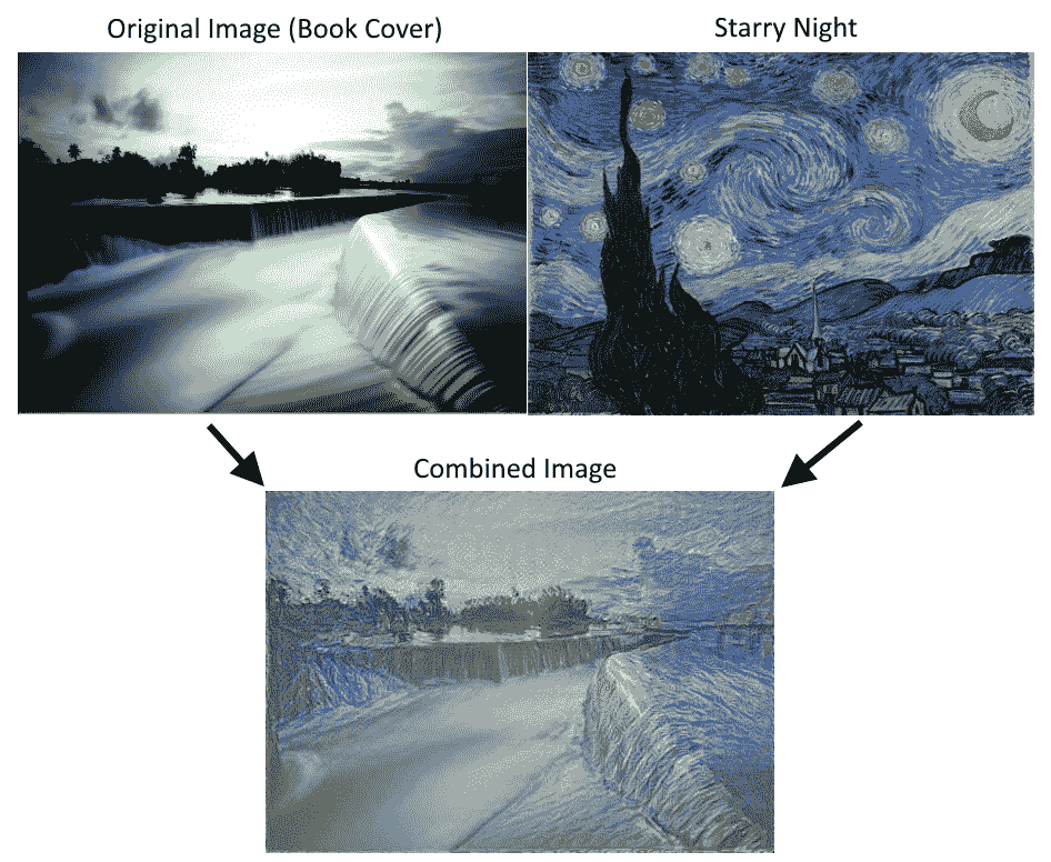圖 6：使用 Stylenet 算法將書籍封面圖像與星夜相結合。請注意，可以通過更改腳本開頭的權重來使用不同的樣式重點 ## 工作原理 我們首先加載兩個圖像，然后將預先訓練的網絡權重和指定的層加載到原始圖像和樣式圖像。我們計算了三種損失函數：原始圖像損失，樣式損失和總變差損失。然后我們訓練隨機噪聲圖片以使用樣式圖像的樣式和原始圖像的內容。 [損失函數受 GitHub 神經風格項目的影響很大](https://github.com/anishathalye/neural-style)。我們還強烈建議讀者查看這些項目中的代碼以獲得改進，更多細節，以及通常更強大的算法，可以提供更好的結果。 ## 另見 * [Gatys，Ecker，Bethge 的藝術風格神經算法，2015](https://arxiv.org/abs/1508.06576) * Leon Gatys 在 CVPR 2016（計算機視覺和模式識別）上的[一個很好的推薦視頻](https://www.youtube.com/watch?v=UFffxcCQMPQ) # 實現 DeepDream 受過訓練的 CNN 的另一個用途是利用一些中間節點檢測標簽特征（例如，貓的耳朵或鳥的羽毛）的事實。利用這一事實，我們可以找到轉換任何圖像的方法，以反映我們選擇的任何節點的節點特征。對于這個秘籍，我們將在 TensorFlow 的網站上瀏覽 DeepDream 教程，但我們將更詳細地介紹基本部分。希望我們可以讓讀者準備好使用 DeepDream 算法來探索 CNN 及其中創建的特征。 ## 準備 TensorFlow 的官方教程展示了如何通過腳本實現 DeepDream（請參閱下一節中的第一個要點）。這個方法的目的是通過他們提供的腳本并解釋每一行。雖然教程很棒，但有些部分可以跳過，有些部分可以使用更多解釋。我們希望提供更詳細的逐行說明。我們還將在必要時使代碼符合 Python3 標準。 ## 操作步驟 執行以下步驟： 1. 為了開始使用 DeepDream，我們需要下載在 CIFAR-1000 上接受過 CNN 訓練的 GoogleNet： ```py me@computer:~$ wget https://storage.googleapis.com/download.tensorflow.org/models/inception5h.zip me@computer:~$ unzip inception5h.zip ``` 1. 我們首先加載必要的庫并啟動圖會話： ```py import os import matplotlib.pyplot as plt import numpy as np import PIL.Image import tensorflow as tf from io import BytesIO graph = tf.Graph() sess = tf.InteractiveSession(graph=graph) ``` 1. 我們現在聲明解壓縮模型參數的位置（從步驟 1 開始）并將參數加載到 TensorFlow 圖中： ```py # Model location model_fn = 'tensorflow_inception_graph.pb' # Load graph parameters with tf.gfile.FastGFile(model_fn, 'rb') as f: graph_def = tf.GraphDef() graph_def.ParseFromString(f.read()) ``` 1. 我們為輸入創建一個占位符，保存 imagenet 平均值 117.0，然后使用正則化占位符導入圖定義： ```py # Create placeholder for input t_input = tf.placeholder(np.float32, name='input') # Imagenet average bias to subtract off images imagenet_mean = 117.0 t_preprocessed = tf.expand_dims(t_input-imagenet_mean, 0) tf.import_graph_def(graph_def, {'input':t_preprocessed}) ``` 1. 接下來，我們將導入卷積層，以便在以后可視化并使用它們進行 DeepDream 處理： ```py # Create a list of layers that we can refer to later layers = [op.name for op in graph.get_operations() if op.type=='Conv2D' and 'import/' in op.name] # Count how many outputs for each layer feature_nums = [int(graph.get_tensor_by_name(name+':0').get_shape()[-1]) for name in layers] ``` 1. 現在我們將選擇一個可視化的層。我們也可以通過名字選擇其他人。我們選擇查看特征號`139`。圖像以隨機噪聲開始： ```py layer = 'mixed4d_3x3_bottleneck_pre_relu' channel = 139 img_noise = np.random.uniform(size=(224,224,3)) + 100.0 ``` 1. 我們聲明了一個繪制圖像數組的函數： ```py def showarray(a, fmt='jpeg'): # First make sure everything is between 0 and 255 a = np.uint8(np.clip(a, 0, 1)*255) # Pick an in-memory format for image display f = BytesIO() # Create the in memory image PIL.Image.fromarray(a).save(f, fmt) # Show image plt.imshow(a) ``` 1. 我們將通過創建一個從圖中按名稱檢索層的函數來縮短一些重復代碼： ```py def T(layer): #Helper for getting layer output tensor return graph.get_tensor_by_name("import/%s:0"%layer) ``` 1. 我們將創建的下一個函數是一個包裝函數，用于根據我們指定的參數創建占位符： ```py # The following function returns a function wrapper that will create the placeholder # inputs of a specified dtype def tffunc(*argtypes): '''Helper that transforms TF-graph generating function into a regular one. See "resize" function below. ''' placeholders = list(map(tf.placeholder, argtypes)) def wrap(f): out = f(*placeholders) def wrapper(*args, **kw): return out.eval(dict(zip(placeholders, args)), session=kw.get('session')) return wrapper return wrap ``` 1. 我們還需要一個將圖像大小調整為大小規格的函數。我們使用 TensorFlow 的內置圖像線性插值函數：`tf.image.resize.bilinear()` ```py # Helper function that uses TF to resize an image def resize(img, size): img = tf.expand_dims(img, 0) # Change 'img' size by linear interpolation return tf.image.resize_bilinear(img, size)[0,:,:,:] ``` 1. 現在我們需要一種方法來更新源圖像，使其更像我們使用的特征。我們通過指定如何計算圖像上的梯度來完成此操作。我們定義了一個函數，用于計算圖像上子區域（圖塊）的梯度，以加快計算速度。為了防止平鋪輸出，我們將在`x`和`y`方向上隨機移動或滾動圖像，這將平滑平鋪效果： ```py def calc_grad_tiled(img, t_grad, tile_size=512): '''Compute the value of tensor t_grad over the image in a tiled way. Random shifts are applied to the image to blur tile boundaries over multiple iterations.''' # Pick a subregion square size sz = tile_size # Get the image height and width h, w = img.shape[:2] # Get a random shift amount in the x and y direction sx, sy = np.random.randint(sz, size=2) # Randomly shift the image (roll image) in the x and y directions img_shift = np.roll(np.roll(img, sx, 1), sy, 0) # Initialize the while image gradient as zeros grad = np.zeros_like(img) # Now we loop through all the sub-tiles in the image for y in range(0, max(h-sz//2, sz),sz): for x in range(0, max(w-sz//2, sz),sz): # Select the sub image tile sub = img_shift[y:y+sz,x:x+sz] # Calculate the gradient for the tile g = sess.run(t_grad, {t_input:sub}) # Apply the gradient of the tile to the whole image gradient grad[y:y+sz,x:x+sz] = g # Return the gradient, undoing the roll operation return np.roll(np.roll(grad, -sx, 1), -sy, 0) ``` 1. 現在我們可以聲明 DeepDream 函數。我們算法的目標是我們選擇的特征的平均值。損耗在梯度上運行，這取決于輸入圖像和所選特征之間的距離。策略是將圖像分成高頻和低頻，并計算低頻部分的梯度。將得到的高頻圖像再次分開并重復該過程。原始圖像和低頻圖像的集合稱為`octaves`。對于每次傳遞，我們計算梯度并將它們應用于圖像： ```py def render_deepdream(t_obj, img0=img_noise, iter_n=10, step=1.5, octave_n=4, octave_scale=1.4): # defining the optimization objective, the objective is the mean of the feature t_score = tf.reduce_mean(t_obj) # Our gradients will be defined as changing the t_input to get closer to the values of t_score. Here, t_score is the mean of the feature we select. # t_input will be the image octave (starting with the last) t_grad = tf.gradients(t_score, t_input)[0] # behold the power of automatic differentiation! # Store the image img = img0 # Initialize the image octave list octaves = [] # Since we stored the image, we need to only calculate n-1 octaves for i in range(octave_n-1): # Extract the image shape hw = img.shape[:2] # Resize the image, scale by the octave_scale (resize by linear interpolation) lo = resize(img, np.int32(np.float32(hw)/octave_scale)) # Residual is hi. Where residual = image - (Resize lo to be hw-shape) hi = img-resize(lo, hw) # Save the lo image for re-iterating img = lo # Save the extracted hi-image octaves.append(hi) # generate details octave by octave for octave in range(octave_n): if octave>0: # Start with the last octave hi = octaves[-octave] # img = resize(img, hi.shape[:2])+hi for i in range(iter_n): # Calculate gradient of the image. g = calc_grad_tiled(img, t_grad) # Ideally, we would just add the gradient, g, but # we want do a forward step size of it ('step'), # and divide it by the avg. norm of the gradient, so # we are adding a gradient of a certain size each step. # Also, to make sure we aren't dividing by zero, we add 1e-7\. img += g*(step / (np.abs(g).mean()+1e-7)) print('.',end = ' ') showarray(img/255.0) ``` 1. 通過我們所做的所有特征設置，我們現在可以運行 DeepDream 算法： ```py # Run Deep Dream if __name__=="__main__": # Create resize function that has a wrapper that creates specified placeholder types resize = tffunc(np.float32, np.int32)(resize) # Open image img0 = PIL.Image.open('book_cover.jpg') img0 = np.float32(img0) # Show Original Image showarray(img0/255.0) # Create deep dream render_deepdream(T(layer)[:,:,:,139], img0, iter_n=15) sess.close() ``` 輸出如下：  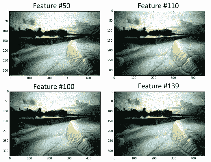圖 7：本書的封面，貫穿 DeepDream 算法，其特征層編號為 50，110，100 和 139 ## 更多 我們敦促讀者使用 DeepDream 官方教程作為進一步信息的來源，并訪問 DeepDream 上的原始 Google 研究博客文章（請參閱下面的第二個要點參見另見部分）。 ## 另見 * [DeepDream 上的 TensorFlow 教程](https://github.com/tensorflow/tensorflow/tree/master/tensorflow/examples/tutorials/deepdream) * [關于 DeepDream 的最初 Google 研究博客文章](https://research.googleblog.com/2015/06/inceptionism-going-deeper-into-neural.html)