# 九、TensorFlow 估計器和 TensorFlow HUB 本章分為兩部分，但是此處的技術是相關的。 首先，我們將研究 TensorFlow 估計器如何為 TensorFlow 提供簡單的高級 API，其次，我們將研究 TensorFlow Hub 如何包含可在自己的應用中使用的模塊。 在本章中，我們將涵蓋以下主要主題： * TensorFlow 估計器 * TensorFlow HUB # TensorFlow 估計器 `tf.estimator`是 TensorFlow 的高級 API。 它通過提供用于服務模型的直接訓練，評估，預測和導出的方法來簡化機器學習編程。 估計器為 TensorFlow 開發人員帶來了許多優勢。 與低級 API 相比，使用估計器開發模型更容易，更直觀。 特別是，同一模型可以在本地計算機或分布式多服務器系統上運行。 該模型也不了解其所處的處理器，即 CPU，GPU 或 TPU。 估計器還通過簡化模型開發人員共享實現的過程，簡化了開發過程，并且由于構建在 Keras 層上，因此使自定義更加簡單。 估計器會處理與 TensorFlow 模型一起使用的所有背景管線。 它們支持安全，分布式的訓練循環，用于圖構建，變量初始化，數據加載，異常處理，創建檢查點文件，從故障中恢復以及為 TensorBoard 保存摘要。 正如我們將看到的，由于它們創建檢查點，因此它們支持在給定數量的步驟之后停止和開始訓練。 開發估計器模型的過程分為四個步驟： 1. 采集數據并創建數據函數 2. 創建特征列 3. 實例化估計器 4. 評估模型的表現 我們將在以下代碼中舉例說明這些步驟。 我們之前已經看過`fashion_mnist`數據集（在第 5 章“將 TensorFlow 2 用于無監督學習”），因此我們將再次使用該數據集來演示估計器的用例。 # 代碼 首先，這是必需的導入： ```py import tensorflow as tf import numpy as np ``` 接下來，我們獲取并預處理數據。 注意，`tf.keras.datasets`中方便地存在`fashion_mnist`。 數據集中的`x`值采用整數 NumPy 數組的形式，每個元素的范圍為 0 到 255，代表`28 x 28`像素時尚圖像中每個像素的灰度值。 為了進行訓練，必須將這些值轉換為 0 到 1 范圍內的浮點數。`y`值采用無符號 8 位整數`(uint8)`的形式，并且必須轉換為 32 位整數（`int32` ），供估計工具再次使用。 盡管可以用以下方法試驗該超參數值，但將學習率設置為一個很小的值： ```py fashion = tf.keras.datasets.fashion_mnist (x_train, y_train),(x_test, y_test) = fashion.load_data() print(type(x_train)) x_train, x_test = x_train / 255.0, x_test / 255.0 y_train, y_test = np.int32(y_train), np.int32(y_test) learning_rate = 1e-4 ``` 之后，是我們的訓練輸入特征。 當您具有數組中的完整數據集并需要快速進行批量，混排和/或重復的方法時，將使用`tf.compat.v1.estimator.inputs.numpy_input_fn`。 其簽名如下： ```py tf.compat.v1.estimator.inputs.numpy_input_fn( x, y=None, batch_size=128, num_epochs=1, shuffle=None, queue_capacity=1000, num_threads=1 ) ``` 將此與我們對函數的調用進行比較，您可以看到`x`值如何作為 NumPy 數組的字典（與張量兼容）傳遞，以及`y`照原樣傳遞。 在此階段，我們尚未指定周期數，即該函數將永遠運行（稍后將指定步驟），我們的批量大小（即一步中顯示的圖像數）為`50`， 并在每一步之前將數據在隊列中混洗。 其他參數保留為其默認值： ```py train_input_fn = tf.compat.v1.estimator.inputs.numpy_input_fn( x={"x": x_train}, y=y_train, num_epochs=None, batch_size=50, shuffle=True ) ``` 值得一提的是，盡管這樣的便利函數雖然在 TensorFlow 2.0 alpha 中不可用，但仍有望改用 TensorFlow2。 測試函數具有相同的簽名，但是在這種情況下，我們僅指定一個周期，并且正如 Google 所建議的那樣，我們不會對數據進行混洗。 同樣，其余參數保留為其默認值： ```py test_input_fn = tf.compat.v1.estimator.inputs.numpy_input_fn( x={"x": x_test}, y=y_test, num_epochs=1, shuffle=False ) ``` 接下來，我們建立特征列。 特征列是一種將數據傳遞給估計器的方法。 特征列函數的簽名如下。 `key`是唯一的字符串，是與我們先前在輸入函數中指定的字典名稱相對應的列名稱（有關不同類型的特征列的更多詳細信息，請參見[這里](https://www.tensorflow.org/api_docs/python/tf/feature_column)）： ```py tf.feature_column.numeric_column( key, shape=(1,), default_value=None, dtype=tf.float32, normalizer_fn=None ) ``` 在我們的特定特征列中，我們可以看到關鍵是`"x"`，并且形狀就是`fashion_mnist`數據集圖像的`28 x 28`像素形狀： ```py feature_columns = [tf.feature_column.numeric_column("x", shape=[28, 28])] ``` 接下來，我們實例化我們的估計器，它將進行分類。 它將為我們構建一個深度神經網絡。 它的簽名很長很詳細，因此我們將帶您參考[這里](https://www.tensorflow.org/api_docs/python/tf/estimator/DNNClassifier)，因為我們將主要使用其默認參數。 它的第一個參數是我們剛剛指定的特征，而第二個參數是我們的網絡規模。 （輸入層和輸出層由估計器在后臺添加。）`AdamOptimizer`是安全的選擇。 `n_classes`對應于我們`fashion_mnist`數據集的`y`標簽數量，我們在其中添加了`0.1`的適度`dropout`。 然后，`model_dir`是我們保存模型參數及其圖和檢查點的目錄。 此目錄還用于將檢查點重新加載到估計器中以繼續訓練： ```py # Build 2 layer DNN classifier classifier = tf.estimator.DNNClassifier( feature_columns=feature_columns, hidden_units=[256, 32], optimizer=tf.compat.v1.train.AdamOptimizer(learning_rate), n_classes=10, dropout=0.1, model_dir="./tmp/mnist_modelx" , loss_reduction=tf.compat.v1.losses.Reduction.SUM) ``` 現在，我們準備訓練模型。 如果您第二次或之后運行`.train`循環，則 Estimator 將從`model_dir`加載其模型參數，并進行進一步的`steps`訓練（要完全從頭開始，只需通過`model_dir`刪除指定的目錄）： ```py classifier.train(input_fn=train_input_fn, steps=10000) ``` 典型的輸出線如下所示： ```py INFO:tensorflow:loss = 25.540459, step = 1600 (0.179 sec) INFO:tensorflow:global_step/sec: 523.471 ``` 最終輸出如下所示： ```py INFO:tensorflow:Saving checkpoints for 10000 into ./tmp/mnist_modelx/model.ckpt. INFO:tensorflow:Loss for final step: 13.06977. 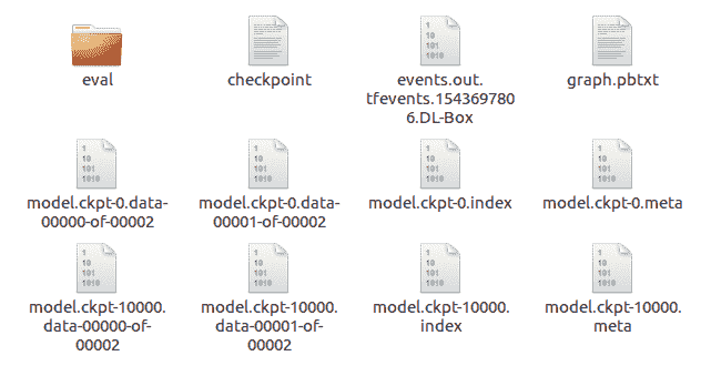``` `model_dir`中指定的目錄如下所示：  為了評估模型的表現，使用了`classifier.evaluate`方法。 其簽名如下： ```py classifier.evaluate(input_fn, steps=None, hooks=None, checkpoint_path=None, name=None) ``` 這將返回一個字典，因此在我們的調用中，我們正在提取準確率指標。 在此，`steps`默認為`None`。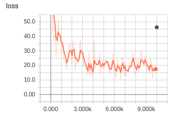 這將評估模型，直到`input_fn`引發輸入結束異常，即，它將評估整個測試集： ```py accuracy_score = classifier.evaluate(input_fn=test_input_fn)["accuracy"] print("\nTest Accuracy: {0:f}%\n".format(accuracy_score*100)) ``` 我們還可以使用以下命令在 TensorBoard 中查看訓練的進度： ```py tensorboard --logdir=./tmp/mnist_modelx ``` 此處，損失圖如下所示，其中`x`軸以 1,000（k）單位表示：  到此結束我們對時尚估計器分類器的了解。 現在我們來看看 TensorFlow Hub。 # TensorFlow HUB TensorFlow Hub 是一個軟件庫。 其目的是提供可重用的組件（稱為模塊），這些組件可在開發組件的原始上下文之外的上下文中使用。 所謂模塊，是指 TensorFlow 圖的一個獨立部分及其權重，可以在其他類似任務中重復使用。 # IMDb（電影評論數據庫） 在本節中，我們將研究一種基于 Google 的應用，該應用在**情感分析**中分析了電影評論的 IMDb 的子集。 該子集由斯坦福大學主持，包含每部電影的評論，以及情感積極性等級為 1 到 4（差）和 7 到 10（好）的情感。 問題在于確定關于每個電影的文本句子中表達的視圖的極性，即針對每個評論，以確定它是正面評論還是負面評論。 我們將在 TensorFlow Hub 中使用一個模塊，該模塊先前已經過訓練以生成單詞嵌入。 詞嵌入是數字的向量，因此具有相似含義的詞也具有類似的向量。 這是監督學習的示例，因為評論的訓練集將使用 IMDB 數據庫提供的陽性值來訓練模型。 然后，我們將在測試集上使用經過訓練的模型，并查看其預測與 IMDB 數據庫中存儲的預測相比如何，從而為我們提供了一種準確率度量。 可以在[這個頁面](http://ai.stanford.edu/~amaas/data/sentiment/)中找到該數據庫論文的引文。 # 數據集 [以下是數據庫隨附的自述文件](http://ai.stanford.edu/~amaas/data/sentiment/)： "The core dataset contains 50,000 reviews split evenly into 25k train and 25k test sets. The overall distribution of labels is balanced (25k pos and 25k neg)." "In the entire collection, no more than 30 reviews are allowed for any given movie because reviews for the same movie tend to have correlated ratings. Further, the train and test sets contain a disjoint set of movies, so no significant performance is obtained by memorizing movie-unique terms and their associated with observed labels. In the labeled train/test sets, a negative review has a score <= 4 out of 10, and a positive review has a score >= 7 out of 10\. 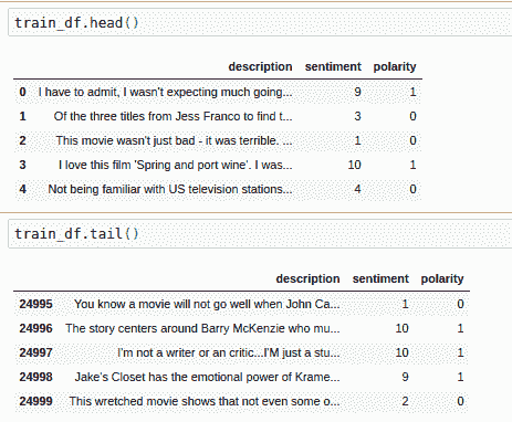Thus, reviews with more neutral ratings are not included in the train/test sets." 這是從 IMDb 訓練頭的頂部起的五行示例： | | **句子** | **情感** | **極性** | | --- | --- | --- | --- | | 0 | `I came here for a review last night before dec...` | 3 | 0 | | 1 | `Look, I'm reading and reading these comments and...` | 4 | 0 | | 2 | `I was overtaken by the emotion. Unforgettable ...` | 10 | 1 | | 3 | `This movie could have been a decent B-movie if...` | 4 | 0 | | 4 | `I have a thing for old black and white movies ...` | 10 | 1 | 這是其尾部的五行： | | 句子 | 情感 | 極性 | | --- | --- | --- | --- | | 24995 | `I have watched some pretty poor films in the p...` | 1 | 0 | | 24996 | `This film is a calculated attempt to cash in t...` | 1 | 0 | | 24997 | `This movie was so very badly written. The char...` | 1 | 0 | | 24998 | `I am a huge Stooges fan but the one and only r...` | 2 | 0 | | 24999 | `Well, let me start off by saying how utterly H...` | 3 | 0 | 以下是測試集：  # 代碼 現在，讓我們看一下在這些數據上訓練的代碼。 在程序的頂部，我們有通常的導入，以及可能需要與`pip` – `tensorflow_hub`，`pandas`和`seaborn`一起安裝的三個額外的導入。 如前所述，我們將使用`tensorflow_hub`中的模塊； 我們還將使用`pandas`的一些`DataFrame`屬性和`seaborn`的一些繪制方法： ```py import tensorflow as tf import tensorflow_hub as hub import matplotlib.pyplot as plt import numpy as np import os import pandas as pd import re import seaborn as sns ``` 另外，這是一些值和我們稍后需要的方法： ```py n_classes = 2 hidden_units = [500,100] learning_rate = 1e-4 steps = 1000 optimizer = tf.optimizers.Adagrad(learning_rate=learning_rate) # upgrade script gave this: #optimizer = tf.compat.v1.train.AdagradOptimizer(learning_rate = learning_rate) ``` 重要的是要認識到，這里使用的 IMDb 數據是目錄的分層結構形式。 頂級 IMDb 目錄包含兩個子目錄：`train`和`test`。 `train`和`test`子目錄分別包含另外兩個子目錄`pos`和`neg`： * `pos`：包含文本文件的集合。 每個文本文件都是正面評價（極性為 1）。 * `neg`：包含文本文件的集合。 每個文本文件都是負面評論（極性為 0）。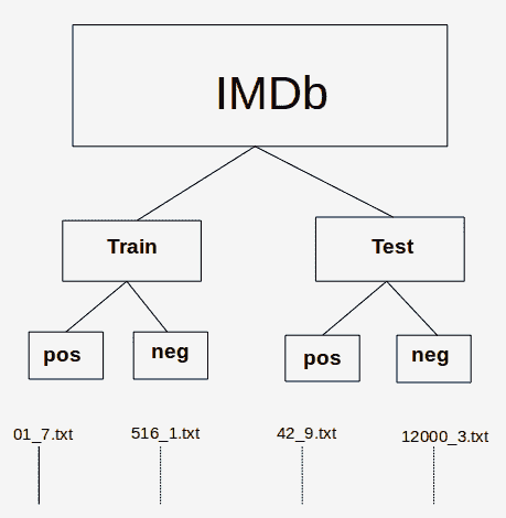 情感（分別為 7 到 10 或 1 到 4）記錄在文件名中； 例如，文件名為`18_7.txt`的文本文件評論的情感為 7（`pos`），而文件名為`38_2.txt`的文本文件評論的情感為 2（`neg`）：  IMDb 目錄/文件層次結構 我們從調用層次結構中的三個函數開始，這些函數獲取并預處理審閱數據。 在第一個函數`load_data(directory)`中，`directory_data`是一個字典，其中加載了`directory`中的數據，該數據作為參數傳入并作為 pandas `DataFrame`返回。 用`description`和`sentiment`鍵初始化`directory_data`字典，然后將它們分配為空列表作為值。 然后，該函數循環遍歷`directory`中的每個文件，并且對于每個文本文件，讀取其內容（作為電影評論）并將其附加到情感列表中。 然后，它使用正則表達式分析文件名并提取數字情感，如前所示，該數字情感緊隨文件名中的下劃線（`_`）。 該函數將此數字情感附加到`sentiment`列表中。 當所有`.txt`文件都循環通過后，該函數將返回已轉換為 pandas `DataFrame`的字典： ```py # Load all files from a directory into a Pandas DataFrame. def load_data(directory): directory_data = {} directory_data["description"] = [] directory_data["sentiment"] = [] for file in os.listdir(directory): with tf.io.gfile.GFile(os.path.join(directory, file), "r") as f: directory_data["description"].append(f.read()) directory_data["sentiment"].append(re.match("\d+_(\d+)\.txt", file).group(1)) return pd.DataFrame.from_dict(directory_data) ``` 如我們前面所述，下一個函數`load(directory)`調用`load_data(directory)`從`pos`和`neg`子目錄創建一個`DataFrame`。 它將適當的極性作為額外字段添加到每個`DataFrame`。 然后，它返回一個新的`DataFrame`，該數據幀由`pos`和`neg`的`DataFrame`的連接組成，經過混洗（`sample(frac=1)`），并插入了新的數字索引（因為我們已經對行進行了混排）： ```py # Merge positive and negative examples, add a polarity column and shuffle. def load(directory): positive_df = load_data(os.path.join(directory, "pos")) positive_df["polarity"] = 1 negative_df = load_data(os.path.join(directory, "neg")) negative_df["polarity"] = 0 return pd.concat([positive_df, negative_df]).sample(frac=1).reset_index(drop=True) ``` 第三個也是最后一個函數是`acquire_data()`。 如果緩存中不存在該函數，則使用 Keras 工具從 Stanford URL 中獲取我們所需的文件。 默認情況下，高速緩存是位于`~/.keras/datasets`的目錄，如有必要，文件將提取到該位置。 該工具將返回到我們的 IMDb 的路徑。 然后將其傳遞給`load_dataset()`的兩個調用，以獲取訓練和測試`DataFrame`： ```py # Download and process the dataset files. def acquire_data(): data = tf.keras.utils.get_file( fname="aclImdb.tar.gz", origin="http://ai.stanford.edu/~amaas/data/sentiment/aclImdb_v1.tar.gz", extract=True) train_df = load(os.path.join(os.path.dirname(data), "aclImdb", "train")) test_df = load(os.path.join(os.path.dirname(data), "aclImdb", "test")) return train_df, test_df tf.compat.v1.logging.set_verbosity(tf.compat.v1.logging.ERROR) ``` 主程序要做的第一件事是通過調用我們剛剛描述的函數來獲取訓練并測試 pandas `DataFrame`： ```py train_df, test_df = acquire_data() ``` 此時，`train_df`和`test_df`包含我們要使用的數據。 在查看下一個片段之前，讓我們看一下它的簽名。 這是一個估計器，它返回用于將 Pandas `DataFrame`饋入模型的輸入函數： ```py tf.compat.v1.estimator.inputs.pandas_input_fn(x, y=None, batch_size=128, num_epochs=1, shuffle=None, queue_capacity=1000, num_threads=1, target_column='target') ``` 調用本身如下： ```py # Training input on the whole training set with no limit on training epochs train_input_fn = tf.compat.v1.estimator.inputs.pandas_input_fn(train_df, train_df["polarity"], num_epochs=None, shuffle=True) ``` 通過將此調用與函數簽名進行比較，我們可以看到訓練數據幀`train_df`與每個評論的極性一起傳入。 `num_epochs =None`表示對訓練周期的數量沒有限制，因為我們將在后面進行指定； `shuffle=True`表示以隨機順序讀取記錄，即文件的每一行。 接下來是預測訓練結果的函數： ```py # Prediction on the whole training set. predict_train_input_fn = tf.compat.v1.estimator.inputs.pandas_input_fn(train_df, train_df["polarity"], shuffle=False) ``` 我們還具有預測測試結果的函數： ```py # Prediction on the test set. predict_test_input_fn = tf.compat.v1.estimator.inputs.pandas_input_fn(test_df, test_df["polarity"], shuffle=False) ``` 然后，我們有特征列。 特征列是原始數據和估計器之間的中介。 共有九種特征列類型。 它們根據其類型采用數值或分類數據，然后將數據轉換為適用于估計器的格式。 在[這個頁面](https://www.tensorflow.org/guide/feature_columns)上有一個出色的描述以及許多示例。 請注意，嵌入來自`tf.hub`： ```py embedded_text_feature_column = hub.text_embedding_column( key="description", module_spec="https://tfhub.dev/google/nnlm-en-dim128/1") ``` 接下來，我們有我們的深度神經網絡估計器。 估計器是用于處理模型的高級工具。 估計器的示例包括`DNNClassifier`，即用于 TensorFlow 深層神經網絡的分類器（在以下代碼中使用），以及`LinearRegressor`，即用于線性回歸問題的分類器。 其簽名如下： ```py tf.estimator.DNNClassifier(hidden_units, feature_columns, model_dir=None, n_classes=2, weight_column=None, label_vocabulary=None, optimizer='Adagrad', activation_fn=<function relu at 0x7fbb75512488>, dropout=None, input_layer_partitioner=None, config=None, warm_start_from=None, loss_reduction='weighted_sum', batch_norm=False, loss_reduction=None) ``` 讓我們將此與通話進行比較： ```py estimator = tf.estimator.DNNClassifier( hidden_units = hidden_units, feature_columns=[embedded_text_feature_column], n_classes=n_classes, optimizer= optimiser, model_dir = "./tmp/IMDbModel" , loss_reduction=tf.compat.v1.losses.Reduction.SUM) ``` 我們可以看到，我們將使用具有 500 和 100 個單元的隱藏層的神經網絡，我們先前定義的特征列，兩個輸出類（標簽）和`ProximalAdagrad`優化器。 請注意，與前面的示例一樣，由于我們指定了`model_dir`，因此估計器將保存一個檢查點和各種模型參數，以便在重新訓練時，將從該目錄加載模型并對其進行進一步的訓練`steps`。 現在，我們可以使用以下代碼來訓練我們的網絡： ```py estimator.train(input_fn=train_input_fn, steps=steps); ``` 此代碼塊為我們的結果造成混淆矩陣。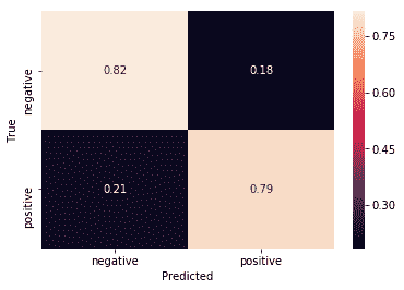 在我們的上下文中，混淆矩陣是一個圖表，顯示了經過訓練的模型的以下內容： * **真陽性**：真實的正面情感被正確地預測為正面的評論（右下） * **真陰性**：真實的負面情感被正確地預測為負面的評論（左上） * **假陽性**：真實的負面情感被錯誤地預測為正面的評論（右上） * **假陰性**：真實的正面情感被錯誤地預測為負面的評論（左下） 以下是我們的訓練集的混淆矩陣：  訓練集的混淆矩陣 原始數據如下： | 9,898 | 2602 | | 2,314 | 10,186 | 注意總數是 25,000，這是我們使用的訓練示例的數量。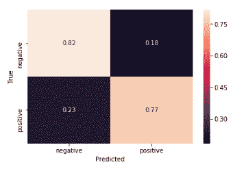 這是我們測試集的混淆矩陣：  測試集的混淆矩陣 原始數據如下： | 9859 | 2641 | | 2500 | 10000 | 對于混淆矩陣，重要的是，對角線的值（左上到右下）要比該對角線的值高得多。 我們可以從混淆矩陣中立即看到，我們的模型在訓練和測試集上都表現良好（如果在測試集上差一些）。 在代碼中，我們首先有一個獲取預測的函數： ```py def get_predictions(estimator, input_fn): return [prediction["class_ids"][0] for prediction in estimator.predict(input_fn=input_fn)] ``` TensorFlow 有一種創建混淆矩陣的方法（如前所述，它們可以顯示在原始圖中）。 其簽名如下： ```py tf.math.confusion_matrix(labels, predictions, num_classes=None, dtype=tf.int32, name=None, weights=None) ``` 在這里，`labels`是真實的標簽。 我們的代碼調用如下方法： ```py confusion_train = tf.math.confusion_matrix(labels=train_df["polarity"], predictions=get_predictions(estimator, predict_train_input_fn)) print("Raw figures:") print(confusion_train.numpy()) ``` 接下來，我們對混淆矩陣進行歸一化，以便其行總計為 1： ```py # Normalize the confusion matrix so that each row sums to 1. top = confusion_train.numpy() bottom = np.sum(top) confusion_train = 2*top/bottom ``` 最后，我們使用`seaborn`方法`heatmap`繪制混淆矩陣。 此方法的簽名很長且很詳細，因此，查看它的最簡單方法是在 Jupyter 筆記本中將光標放在`Shift + TAB`上。 我們在這里只需要四個參數： ```py sns.heatmap(confusion_train, annot=True, xticklabels=LABELS, yticklabels=LABELS) plt.xlabel("Predicted") plt.ylabel("True") ``` 在這里，我們得到以下內容： ```py LABELS = ["negative", "positive"] ``` 除了使用測試集代替訓練集之外，用于顯示測試集的混淆矩陣的代碼是相同的： ```py # Create a confusion matrix on test data. confusion_test = tf.math.confusion_matrix(labels=test_df["polarity"], predictions=get_predictions(estimator, predict_test_input_fn)) print(confusion_test.numpy()) # Normalize the confusion matrix so that each row sums to 1. top = confusion_test.numpy() bottom = np.sum(top) confusion_test = 2*top/bottom sns.heatmap(confusion_test, annot=True, xticklabels=LABELS, yticklabels=LABELS); plt.xlabel("Predicted"); plt.ylabel("True"); ``` 到此結束我們對 IMDb 情感分析的研究。 # 總結 在本章中，我們介紹了用于訓練時裝數據集的估計器。 我們了解了估計器如何為 TensorFlow 提供簡單直觀的 API。 然后，我們查看了另一個應用，這一次是對 IMDb 中電影評論的情感分類。 我們看到了 TensorFlow Hub 如何為我們提供文本嵌入，即單詞的向量，這是具有相似含義的單詞具有相似向量的地方。 在本書中，我們看到了 TensorFlow 2.0 alpha 的概述。