# 二、在 Eager 模式中使用指標 大家好！ 在本教程中，我們將學習如何使用各種指標來評估在 TensorFlow 中使用 Eager 模式時神經網絡的表現。 我玩了很久 TensorFlow Eager 模式，我喜歡它。對我來說，與使用聲明模式相比，API 看起來非常直觀，現在一切看起來都更容易構建。 我現在發現的主要不便之處（我使用的是 1.7 版）是使用 Eager 模式時，`tf.metrics`還不兼容。 盡管如此，我已經構建了幾個函數，可以幫助你評估網絡的表現，同時仍然享受憑空構建網絡的強大之處。 教程步驟：  我選擇了三個案例： 多分類 對于此任務，我們將使用準確率，混淆矩陣和平均精度以及召回率，來評估我們模型的表現。 不平衡的二分類 當我們處理不平衡的數據集時，模型的準確率不是可靠的度量。 因此，我們將使用 ROC-AUC 分數，這似乎是一個更適合不平衡問題的指標。 回歸 為了評估我們的回歸模型的性能，我們將使用 R ^ 2 分數（確定系數）。 我相信這些案例的多樣性足以幫助你進一步學習任何機器學習項目。 如果你希望我添加下面未遇到的任何額外指標，請告知我們，我會盡力在以后添加它們。 那么，讓我們開始吧！ TensorFlow 版本 - 1.7 ## 導入重要的庫并開啟 Eager 模式 ```py # 導入 TensorFlow 和 TensorFlow Eager import tensorflow as tf import tensorflow.contrib.eager as tfe # 導入函數來生成玩具分類問題 from sklearn.datasets import load_wine from sklearn.datasets import make_classification from sklearn.datasets import make_regression # 為數據預處理導入 numpy import numpy as np # 導入繪圖庫 import matplotlib.pyplot as plt %matplotlib inline # 為降維導入 PCA from sklearn.decomposition import PCA # 開啟 Eager 模式。一旦開啟不能撤銷！只執行一次。 tfe.enable_eager_execution() ``` ## 第一部分：用于多分類的的數據集 ```py wine_data = load_wine() print('Type of data in the wine_data dictionary: ', list(wine_data.keys())) ''' Type of data in the wine_data dictionary: ['data', 'target', 'target_names', 'DESCR', 'feature_names'] ''' print('Number of classes: ', len(np.unique(wine_data.target))) # Number of classes: 3 print('Distribution of our targets: ', np.unique(wine_data.target, return_counts=True)[1]) # Distribution of our targets: [59 71 48] print('Number of features in the dataset: ', wine_data.data.shape[1]) # Number of features in the dataset: 13 ``` ### 特征標準化 每個特征的比例變化很大，如下面的單元格所示。 為了加快訓練速度，我們將每個特征標準化為零均值和單位標準差。 這個過程稱為標準化，它對神經網絡的收斂非常有幫助。 ```py # 數據集標準化 wine_data.data = (wine_data.data - np.mean(wine_data.data, axis=0))/np.std(wine_data.data, axis=0) print('Standard deviation of each feature after standardization: ', np.std(wine_data.data, axis=0)) # Standard deviation of each feature after standardization: [1. 1. 1. 1. 1. 1. 1. 1. 1. 1. 1. 1. 1.] ``` ### 數據可視化：使用 PCA 降到二維 我們將使用 PCA，僅用于可視化目的。 我們將使用所有 13 個特征來訓練我們的神經網絡。 讓我們看看這三個類如何在 2D 空間中表示。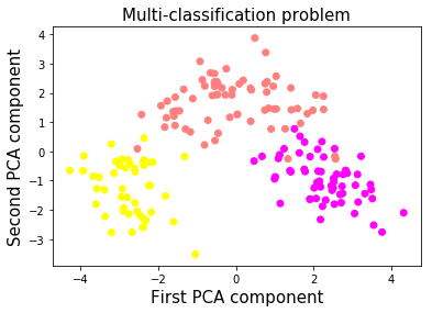 ```py X_pca = PCA(n_components=2, random_state=2018).fit_transform(wine_data.data) plt.scatter(X_pca[:,0], X_pca[:,1], c=wine_data.target, cmap=plt.cm.spring) plt.xlabel('First PCA component', fontsize=15) plt.ylabel('Second PCA component', fontsize=15) plt.title('Multi-classification problem', fontsize=15) plt.show() ```  好的，所以這些類看起來很容易分開。 順便說一句，我實際上在特征標準化之前嘗試使用 PCA，粉色和黃色類重疊。 通過在降維之前標準化特征，我們設法在它們之間獲得了清晰的界限。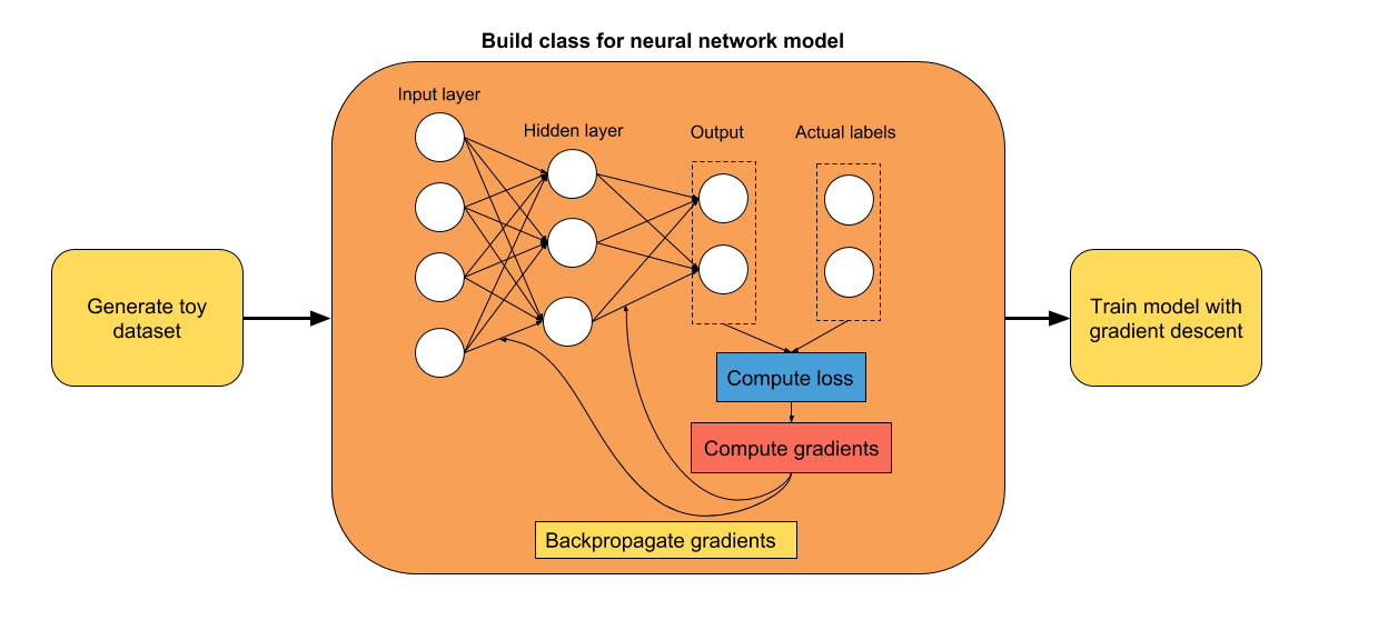 ### 讓我們使用 TensorFlow Eager API 構建雙層神經網絡 你可能已經注意到，使用 TensorFlow Eager 構建模型的最方便方法是使用類。 我認為，為模型使用類可以更容易地組織和添加新組件。 你只需定義初始化期間要使用的層，然后在預測期間使用它們。 它使得在預測階段更容易閱讀模型的架構。 ```py class two_layer_nn(tf.keras.Model): def __init__(self, output_size=2, loss_type='cross-entropy'): super(two_layer_nn, self).__init__() """ 在這里定義正向傳播期間 使用的神經網絡層 Args: output_size: int (default=2). loss_type: string, 'cross-entropy' or 'regression' (default='cross-entropy') """ # 第一個隱層 self.dense_1 = tf.layers.Dense(20, activation=tf.nn.relu) # 第二個隱層 self.dense_2 = tf.layers.Dense(10, activation=tf.nn.relu) # 輸出層，未縮放的對數概率 self.dense_out = tf.layers.Dense(output_size, activation=None) # 初始化損失類型 self.loss_type = loss_type def predict(self, input_data): """ 在神經網絡上執行正向傳播 Args: input_data: 2D tensor of shape (n_samples, n_features). Returns: logits: unnormalized predictions. """ layer_1 = self.dense_1(input_data) layer_2 = self.dense_2(layer_1) logits = self.dense_out(layer_2) return logits def loss_fn(self, input_data, target): """ 定義訓練期間使用的損失函數 """ preds = self.predict(input_data) if self.loss_type=='cross-entropy': loss = tf.losses.sparse_softmax_cross_entropy(labels=target, logits=preds) else: loss = tf.losses.mean_squared_error(target, preds) return loss def grads_fn(self, input_data, target): """ 在每個正向步驟中， 動態計算損失值對模型參數的梯度 """ with tfe.GradientTape() as tape: loss = self.loss_fn(input_data, target) return tape.gradient(loss, self.variables) def fit(self, input_data, target, optimizer, num_epochs=500, verbose=50, track_accuracy=True): """ 用于訓練模型的函數， 使用所選的優化器，執行所需數量的迭代 """ if track_accuracy: # Initialize list to store the accuracy of the model self.hist_accuracy = [] # Initialize class to compute the accuracy metric accuracy = tfe.metrics.Accuracy() for i in range(num_epochs): # Take a step of gradient descent grads = self.grads_fn(input_data, target) optimizer.apply_gradients(zip(grads, self.variables)) if track_accuracy: # Predict targets after taking a step of gradient descent logits = self.predict(X) preds = tf.argmax(logits, axis=1) # Compute the accuracy accuracy(preds, target) # Get the actual result and add it to our list self.hist_accuracy.append(accuracy.result()) # Reset accuracy value (we don't want to track the running mean accuracy) accuracy.init_variables() ``` ### 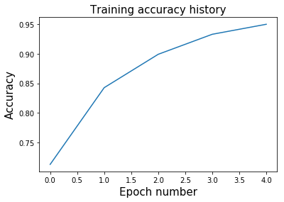準確率指標 為了使用準確率指標評估模型的表現，我們將使用`tfe.metrics.Accuracy`類。 在批量訓練模型時，此指標非常有用，因為它會在每次調用時計算批量的平均精度。 當我們在每個步驟中使用整個數據集訓練模型時，我們將重置此指標，因為我們不希望它跟蹤運行中的平均值。 ```py # 創建輸入特征和標簽。將數據從 numpy 轉換為張量 X = tf.constant(wine_data.data) y = tf.constant(wine_data.target) # 定義優化器 optimizer = tf.train.GradientDescentOptimizer(5e-1) # 初始化模型 model = two_layer_nn(output_size=3) # 在這里選擇迭代數量 num_epochs = 5 # 使用梯度下降訓練模型 model.fit(X, y, optimizer, num_epochs=num_epochs) plt.plot(range(num_epochs), model.hist_accuracy); plt.xlabel('Epoch number', fontsize=15); plt.ylabel('Accuracy', fontsize=15); plt.title('Training accuracy history', fontsize=15); ```  ### 混淆矩陣 在訓練完算法后展示混淆矩陣是一種很好的方式，可以全面了解網絡表現。 TensorFlow 具有內置函數來計算混淆矩陣，幸運的是它與 Eager 模式兼容。 因此，讓我們可視化此數據集的混淆矩陣。 ```py # 獲得整個數據集上的預測 logits = model.predict(X) preds = tf.argmax(logits, axis=1) # 打印混淆矩陣 conf_matrix = tf.confusion_matrix(y, preds, num_classes=3) print('Confusion matrix: \n', conf_matrix.numpy()) ''' Confusion matrix: [[56 3 0] [ 2 66 3] [ 0 1 47]] ''' ``` 對角矩陣顯示真正例，而矩陣的其它地方顯示假正例。 ### 精準率得分 上面計算的混淆矩陣使得計算平均精確率非常容易。 我將在下面實現一個函數，它會自動為你計算。 你還可以指定每個類的權重。 例如，由于某些原因，第二類的精確率可能對你來說更重要。 ```py def precision(labels, predictions, weights=None): conf_matrix = tf.confusion_matrix(labels, predictions, num_classes=3) tp_and_fp = tf.reduce_sum(conf_matrix, axis=0) tp = tf.diag_part(conf_matrix) precision_scores = tp/(tp_and_fp) if weights: precision_score = tf.multiply(precision_scores, weights)/tf.reduce_sum(weights) else: precision_score = tf.reduce_mean(precision_scores) return precision_score precision_score = precision(y, preds, weights=None) print('Average precision: ', precision_score.numpy()) # Average precision: 0.9494581280788177 ``` ### 召回率得分 平均召回率的計算與精確率非常相似。 我們不是對列進行求和，而是對行進行求和，來獲得真正例和假負例的總數。 ```py def recall(labels, predictions, weights=None): conf_matrix = tf.confusion_matrix(labels, predictions, num_classes=3) tp_and_fn = tf.reduce_sum(conf_matrix, axis=1) tp = tf.diag_part(conf_matrix) recall_scores = tp/(tp_and_fn) if weights: recall_score = tf.multiply(recall_scores, weights)/tf.reduce_sum(weights) else: recall_score = tf.reduce_mean(recall_scores) return recall_score recall_score = recall(y, preds, weights=None) print('Average precision: ', recall_score.numpy()) # Average precision: 0.9526322246094269 ``` ## 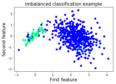第二部分：不平衡二分類 當你開始使用真實數據集時，你會很快發現大多數問題都是不平衡的。 例如，考慮到異常樣本與正常樣本的比例，異常檢測問題嚴重不平衡。 在這些情況下，評估網絡性能的更合適的指標是 ROC-AUC 得分。 那么，讓我們構建我們的不平衡數據集并開始研究它！ ```py XX,, yy == make_classificationmake_cla (n_samples=1000, n_features=2, n_informative=2, n_redundant=0, n_classes=2, n_clusters_per_class=1, flip_y=0.1, class_sep=4, hypercube=False, shift=0.0, scale=1.0, random_state=2018) # 減少標簽為 1 的樣本數 X = np.vstack([X[y==0], X[y==1][:50]]) y = np.hstack([y[y==0], y[y==1][:50]]) ```  我們將使用相同的神經網絡架構。 我們只需用`num_classes = 2`初始化模型，因為我們正在處理二分類問題。 ```py # Numpy 數組變為張量 X = tf.constant(X) y = tf.constant(y) ``` 讓我們將模型只訓練幾個迭代，來避免過擬合。 ```py # 定義優化器 optimizer = tf.train.GradientDescentOptimizer(5e-1) # 初始化模型 model = two_layer_nn(output_size=2) # 在這里選擇迭代數量 num_epochs = 5 # 使用梯度下降訓練模型 model.fit(X, y, optimizer, num_epochs=num_epochs) ``` ### 如何計算 ROC-AUC 得分 為了計算 ROC-AUC 得分，我們將使用`tf.metric.auc`的相同方法。 對于每個概率閾值，我們將計算真正例，真負例，假正例和假負例的數量。 在計算這些統計數據后，我們可以計算每個概率閾值的真正例率和真負例率。 為了近似 ROC 曲線下的面積，我們將使用黎曼和和梯形規則。 如果你想了解更多信息，請點擊[此處](https://www.khanacademy.org/math/ap-calculus-ab/ab-accumulation-riemann-sums/ab-midpoint-trapezoid/a/understanding-the-trapezoid-rule)。 ### ROC-AUC 函數 ```py def roc_auc(labels, predictions, thresholds, get_fpr_tpr=True): tpr = [] fpr = [] for th in thresholds: # 計算真正例數量 tp_cases = tf.where((tf.greater_equal(predictions, th)) & (tf.equal(labels, 1))) tp = tf.size(tp_cases) # 計算真負例數量 tn_cases = tf.where((tf.less(predictions, th)) & (tf.equal(labels, 0))) tn = tf.size(tn_cases) # 計算假正例數量 fp_cases = tf.where((tf.greater_equal(predictions, th)) & (tf.equal(labels,0))) fp = tf.size(fp_cases) # 計算假負例數量 fn_cases = tf.where((tf.less(predictions, th)) & (tf.equal(labels,1))) fn = tf.size(fn_cases) # 計算該閾值的真正例率 tpr_th = tp/(tp + fn) # 計算該閾值的假正例率 fpr_th = fp/(fp + tn) # 附加到整個真正例率列表 tpr.append(tpr_th) # 附加到整個假正例率列表 fpr.append(fpr_th) # 使用黎曼和和梯形法則，計算曲線下的近似面積 auc_score = 0 for i in range(0, len(thresholds)-1): height_step = tf.abs(fpr[i+1]-fpr[i]) b1 = tpr[i] b2 = tpr[i+1] step_area = height_step*(b1+b2)/2 auc_score += step_area return auc_score, fpr, tpr ``` ### 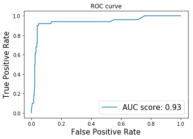為我們訓練的模型計算 ROC-AUC 得分并繪制 ROC 曲線 ```py # 閾值更多意味著曲線下的近似面積的粒度更高 # 隨意嘗試閾值的數量 num_thresholds = 1000 thresholds = tf.lin_space(0.0, 1.0, num_thresholds).numpy() # 將Softmax應用于我們的預測，因為模型的輸出是非標準化的 # 選擇我們的正類的預測（樣本較少的類） preds = tf.nn.softmax(model.predict(X))[:,1] # 計算 ROC-AUC 得分并獲得每個閾值的 TPR 和 FPR auc_score, fpr_list, tpr_list = roc_auc(y, preds, thresholds) print('ROC-AUC score of the model: ', auc_score.numpy()) # ROC-AUC score of the model: 0.93493986 plt.plot(fpr_list, tpr_list, label='AUC score: %.2f' %auc_score); plt.xlabel('False Positive Rate', fontsize=15); plt.ylabel('True Positive Rate', fontsize=15); plt.title('ROC curve'); plt.legend(fontsize=15); ```  ## 第三部分：用于回歸的數據集 我們最終的數據集為簡單的回歸任務而創建。 在前兩個問題中，網絡的輸出表示樣本所屬的類。這里網絡的輸出是連續的，是一個實數。 我們的輸入數據集僅包含一個特征，以便使繪圖保持簡單。 標簽`y`是實數向量。 讓我們創建我們的玩具數據集！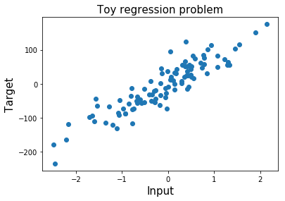 ```py X, y = make_regression(n_samples=100, n_features=1, n_informative=1, noise=30, random_state=2018) ``` ### 展示輸入特征和標簽 為了更好地了解我們正在處理的問題，讓我們繪制標簽和輸入特征。 ```py pltplt..scatterscatter((XX,, yy);); pltplt..xlabelxlabel(('Input''Input',, fontsizefontsize=15); plt.ylabel('Target', fontsize=15); plt.title('Toy regression problem', fontsize=15); ```  ```py # Numpy 數組轉為張量 X = tf.constant(X) y = tf.constant(y) y = tf.reshape(y, [-1,1]) # 從行向量變為列向量 ``` ### 用于回歸任務的神經網絡 我們可以重復使用上面創建的雙層神經網絡。 由于我們只需要預測一個實數，因此網絡的輸出大小為 1。 我們必須重新定義我們的損失函數，因為我們無法繼續使用`softmax`交叉熵損失。 相反，我們將使用均方誤差損失函數。 我們還將定義一個新的優化器，其學習速率比前一個更小。 隨意調整迭代的數量。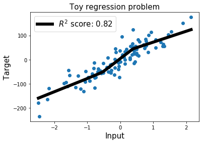 ```py # 定義優化器 optimizer = tf.train.GradientDescentOptimizer(1e-4) # 初始化模型 model = two_layer_nn(output_size=1, loss_type='regression') # 選擇迭代數量 num_epochs = 300 # 使用梯度下降訓練模型 model.fit(X, y, optimizer, num_epochs=num_epochs, track_accuracy=False) ``` ### 計算 R^2 得分（決定系數） 如果你曾經處理過回歸問題，那么你可能已經聽說過這個得分。 這個指標計算輸入特征與目標之間的變異百分率，由我們的模型解釋。R^2 得分的值范圍介于 0 和 1 之間。R^2 得分為 1 意味著該模型可以進行完美的預測。 始終預測目標`y`的平均值，R^2 得分為 0。 R^2 可能為的負值。 在這種情況下，這意味著比起總是預測目標變量的平均值的模型，我們的模型做出更糟糕的預測。 由于此度量標準在 TensorFlow 1.5 中不易獲得，因此在 Eager 模式下運行時，我在下面的單元格中為它創建了一個小函數。 ```py # 計算 R^2 得分 def r2(labels, predictions): mean_labels = tf.reduce_mean(labels) total_sum_squares = tf.reduce_sum((labels-mean_labels)**2) residual_sum_squares = tf.reduce_sum((labels-predictions)**2) r2_score = 1 - residual_sum_squares/total_sum_squares return r2_score preds = model.predict(X) r2_score = r2(y, preds) print('R2 score: ', r2_score.numpy()) # R2 score: 0.8249999999348803 ``` ### 展示最佳擬合直線 為了可視化我們的神經網絡的最佳擬合直線，我們簡單地選取`X_min`和`X_max`之間的線性空間。 ```py # 創建 X_min 和 X_max 之間的數據點來顯示最佳擬合直線 X_best_fit = np.arange(X.numpy().min(), X.numpy().max(), 0.001)[:,None] # X_best_fit 的預測 preds_best_fit = model.predict(X_best_fit) plt.scatter(X.numpy(), y.numpy()); # 原始數據點 plt.plot(X_best_fit, preds_best_fit.numpy(), color='k', linewidth=6, label='$R^2$ score: %.2f' %r2_score) # Our predictions plt.xlabel('Input', fontsize=15); plt.ylabel('Target', fontsize=15); plt.title('Toy regression problem', fontsize=15); plt.legend(fontsize=15); ```