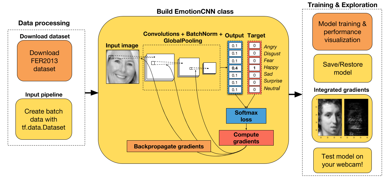
# 七、使用 TensorFlow Eager 構建用于情感識別的卷積神經網絡（CNN） 對于深度學習，我最喜歡的部分之一就是我可以解決一些問題，其中我自己可以測試神經網絡。 到目前為止，我建立的最有趣的神經網絡是用于情感識別的 CNN。 我已經設法通過網絡傳遞我的網絡攝像頭視頻，并實時預測了我的情緒（使用 GTX-1070）。 相當容易上癮！ 因此，如果你想將工作與樂趣結合起來，那么你一定要仔細閱讀本教程。 另外，這是熟悉 Eager API 的好方法！ 教程步驟  + 下載并處理 Kaggle 上提供的 FER2013 數據集。 + 整個數據集上的探索性數據分析。 + 將數據集拆分為訓練和開發數據集。 + 標準化圖像。 + 使用`tf.data.Dataset` API 遍歷訓練和開發數據集。 + 在 Eager 模式下為 CNN 創建一個類。 + 能夠保存模型或從先前的檢查點恢復。 + 創建一個損失函數，一個優化器和一個梯度計算函數。 + 用梯度下降訓練模型。 + 從頭開始或者從預訓練模型開始。 + 在訓練期間可視化表現并計算準確率。 + 使用集成梯度可視化樣本圖像上的 CNN 歸屬。 + 使用 OpenCV 和 Haar 級聯算法在新圖像上測試 CNN。 ## 導入有用的庫 ```py # 導入 TensorFlow 和 TensorFlow Eager import tensorflow as tf import tensorflow.contrib.eager as tfe # 導入函數來生成玩具分類問題 from sklearn.datasets import make_moons import numpy as np # 導入繪圖庫 import matplotlib.pyplot as plt %matplotlib inline # 開啟 Eager 模式。一旦開啟不能撤銷！只執行一次。 tfe.enable_eager_execution() ``` ## 下載數據集 為了訓練我們的 CNN，我們將使用 Kaggle 上提供的 FER2013 數據集。 你必須在他們的平臺上自己下載數據集，遺憾的是我無法公開分享數據。 盡管如此，數據集只有 96.4 MB，因此你應該能夠立即下載它。 你可以在[這里](https://www.kaggle.com/c/challenges-in-representation-learning-facial-expression-recognition-challenge/data)下載。 下載完數據后，將其解壓縮并放入名為`datasets`的文件夾中，這樣你就不必對下面的代碼進行任何修改。 好的，讓我們開始探索性數據分析！ ## 探索性數據分析 在構建任何機器學習模型之前，建議對數據集進行探索性數據分析。 這使你有機會發現數據集中的任何缺陷，如類之間的強烈不平衡，低質量圖像等。 我發現機器學習項目中出現的大多數錯誤，都是由于數據處理不正確造成的。 如果你在發現模型沒有用后才開始調查數據集，那么找到這些錯誤會更加困難。 所以，我給你的建議是：在構建任何模型之前總是分析數據。 ```py # 讀取輸入數據。假設已經解壓了數據集，并放入名為 data 的文件夾中。 path_data = 'datasets/fer2013/fer2013.csv' data = pd.read_csv(path_data) print('Number of samples in the dataset: ', data.shape[0]) # Number of samples in the dataset: 35887 # 查看前五行 data.head(5) ``` | | emotion | pixels | Usage | | --- | --- | --- | --- | | 0 | 0 | 70 80 82 72 58 58 60 63 54 58 60 48 89 115 121... | Training | | 1 | 0 | 151 150 147 155 148 133 111 140 170 174 182 15... | Training | | 2 | 2 | 231 212 156 164 174 138 161 173 182 200 106 38... | Training | | 3 | 4 | 24 32 36 30 32 23 19 20 30 41 21 22 32 34 21 1... | Training | | 4 | 6 | 4 0 0 0 0 0 0 0 0 0 0 0 3 15 23 28 48 50 58 84... | Training | ```py # 獲取每個表情的含義 emotion_cat = {0:'Angry', 1:'Disgust', 2:'Fear', 3:'Happy', 4:'Sad', 5:'Surprise', 6:'Neutral'} # 查看標簽分布（檢查不平衡） target_counts = data['emotion'].value_counts().reset_index(drop=False) target_counts.columns = ['emotion', 'number_samples'] target_counts['emotion'] = target_counts['emotion'].map(emotion_cat) target_counts ``` | | emotion | number_samples | | --- | --- | --- | | 0 | Happy | 8989 | | 1 | Neutral | 6198 | | 2 | Sad | 6077 | | 3 | Fear | 5121 | | 4 | Angry | 4953 | | 5 | Surprise | 4002 | | 6 | Disgust | 547 | 如你所見，數據集非常不平衡。 特別是對于情緒`Disgust`。 這將使這個類的訓練更加困難，因為網絡將有更少的機會來學習這種表情的表示。 在我們訓練網絡之后，稍后我們會看到這是否會嚴重影響我們網絡的訓練。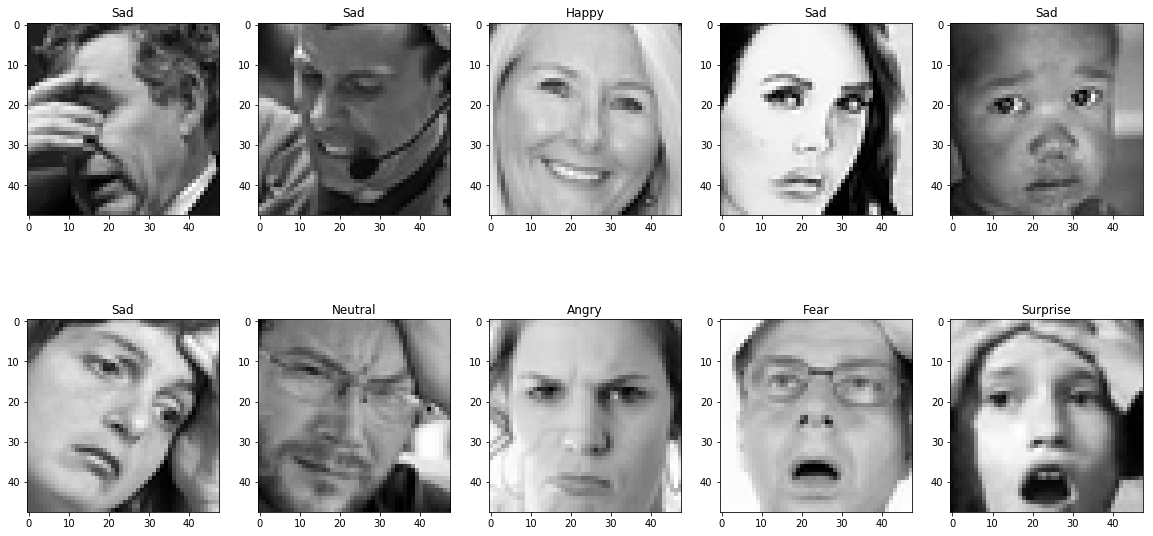 我們來看看一些圖片！ 圖像當前表示為整數的字符串，每個整數表示一個像素的強度。 我們將處理字符串。將其表示為整數列表。 ```py # 將圖像從字符串換換位整數列表 data['pixels'] = data['pixels'].apply(lambda x: [int(pixel) for pixel in x.split()]) # 修改這里的種子來查看其它圖像 random_seed = 2 # 隨機選擇十個圖像 data_sample = data.sample(10, random_state=random_seed) # 為圖像創建子圖 f, axarr = plt.subplots(2, 5, figsize=(20, 10)) # 繪制圖像 i, j = 0, 0 for idx, row in data_sample.iterrows(): img = np.array(row['pixels']).reshape(48,48) axarr[i,j].imshow(img, cmap='gray') axarr[i,j].set_title(emotion_cat[row['emotion']]) if j==4: i += 1 j = 0 else: j += 1 ```  ## 將數據集拆分為訓練/開發，并按最大值標準化圖像 ```py data_traindata_tra = data[data['Usage']=='Training'] size_train = data_train.shape[0] print('Number samples in the training dataset: ', size_train) data_dev = data[data['Usage']!='Training'] size_dev = data_dev.shape[0] print('Number samples in the development dataset: ', size_dev) ''' Number samples in the training dataset: 28709 Number samples in the development dataset: 7178 ''' # 獲取訓練輸入和標簽 X_train, y_train = data_train['pixels'].tolist(), data_train['emotion'].as_matrix() # 將圖像形狀修改為 4D（樣本數，寬，高，通道數） X_train = np.array(X_train, dtype='float32').reshape(-1,48,48,1) # 使用最大值標準化圖像（最大像素密度為 255） X_train = X_train/255.0 # 獲取開發輸入和標簽 X_dev, y_dev = data_dev['pixels'].tolist(), data_dev['emotion'].as_matrix() # 將圖像形狀修改為 4D（樣本數，寬，高，通道數） X_dev = np.array(X_dev, dtype='float32').reshape(-1,48,48,1) # 使用最大值標準化圖像 X_dev = X_dev/255.0 ``` ## 使用`tf.data.Dataset` API 為了準備我們的數據集用作 CNN 的輸入，我們將使用`tf.data.Dataset` API，將我們剛剛創建的 numpy 數組轉換為 TF 張量。 由于此數據集比以前教程中的數據集大得多，因此我們實際上必須將數據批量提供給模型。 通常，為了提高計算效率，你可以選擇與內存一樣大的批量。 但是，根據我的經驗，如果我在訓練期間使用較小的批量，我會在測試數據上獲得更好的結果。 隨意調整批量大小，看看你是否得到了與我相同的結論。 ```py # 隨意調整批量大小 # 通常較小的批量大小在測試集上獲取更好的結果 batch_size = 64 training_data = tf.data.Dataset.from_tensor_slices((X_train, y_train[:,None])).batch(batch_size) eval_data = tf.data.Dataset.from_tensor_slices((X_dev, y_dev[:,None])).batch(batch_size) ``` ## 在 Eager 模式下創建 CNN 模型 CNN 架構在下面的單元格中創建。 如你所見，`EmotionRecognitionCNN`類繼承自`tf.keras.Model`類，因為我們想要跟蹤包含任何可訓練參數的層（例如卷積的權重，批量標準化層的平均值）。 這使我們易于保存這些變量，然后在我們想要繼續訓練網絡時將其恢復。 這個 CNN 的原始架構可以在這里找到（使用 keras 構建）。 我認為如果你開始使用比 ResNet 更簡單的架構，那將非常有用。 對于這個網絡規模，它的效果非常好。 你可以使用它，添加更多的層，增加層的數量，過濾器等。看看你是否可以獲得更好的結果。 有一點可以肯定的是，dropout 越高，網絡效果越好。 ```py class EmotionRecognitionCNN(tf.keras.Model): def __init__(self, num_classes, device='cpu:0', checkpoint_directory=None): ''' 定義在正向傳播期間使用的參數化層，你要在它上面運行計算的設備，以及檢查點目錄。 Args: num_classes: the number of labels in the network. device: string, 'cpu:n' or 'gpu:n' (n can vary). Default, 'cpu:0'. checkpoint_directory: the directory where you would like to save or restore a model. ''' super(EmotionRecognitionCNN, self).__init__() # 初始化層 self.conv1 = tf.layers.Conv2D(16, 5, padding='same', activation=None) self.batch1 = tf.layers.BatchNormalization() self.conv2 = tf.layers.Conv2D(16, 5, 2, padding='same', activation=None) self.batch2 = tf.layers.BatchNormalization() self.conv3 = tf.layers.Conv2D(32, 5, padding='same', activation=None) self.batch3 = tf.layers.BatchNormalization() self.conv4 = tf.layers.Conv2D(32, 5, 2, padding='same', activation=None) self.batch4 = tf.layers.BatchNormalization() self.conv5 = tf.layers.Conv2D(64, 3, padding='same', activation=None) self.batch5 = tf.layers.BatchNormalization() self.conv6 = tf.layers.Conv2D(64, 3, 2, padding='same', activation=None) self.batch6 = tf.layers.BatchNormalization() self.conv7 = tf.layers.Conv2D(64, 1, padding='same', activation=None) self.batch7 = tf.layers.BatchNormalization() self.conv8 = tf.layers.Conv2D(128, 3, 2, padding='same', activation=None) self.batch8 = tf.keras.layers.BatchNormalization() self.conv9 = tf.layers.Conv2D(256, 1, padding='same', activation=None) self.batch9 = tf.keras.layers.BatchNormalization() self.conv10 = tf.layers.Conv2D(128, 3, 2, padding='same', activation=None) self.conv11 = tf.layers.Conv2D(256, 1, padding='same', activation=None) self.batch11 = tf.layers.BatchNormalization() self.conv12 = tf.layers.Conv2D(num_classes, 3, 2, padding='same', activation=None) # 定義設備 self.device = device # 定義檢查點目錄 self.checkpoint_directory = checkpoint_directory def predict(self, images, training): """ 根據輸入樣本預測每個類的概率。 Args: images: 4D tensor. Either an image or a batch of images. training: Boolean. Either the network is predicting in training mode or not. """ x = self.conv1(images) x = self.batch1(x, training=training) x = self.conv2(x) x = self.batch2(x, training=training) x = tf.nn.relu(x) x = tf.layers.dropout(x, rate=0.4, training=training) x = self.conv3(x) x = self.batch3(x, training=training) x = self.conv4(x) x = self.batch4(x, training=training) x = tf.nn.relu(x) x = tf.layers.dropout(x, rate=0.3, training=training) x = self.conv5(x) x = self.batch5(x, training=training) x = self.conv6(x) x = self.batch6(x, training=training) x = tf.nn.relu(x) x = tf.layers.dropout(x, rate=0.3, training=training) x = self.conv7(x) x = self.batch7(x, training=training) x = self.conv8(x) x = self.batch8(x, training=training) x = tf.nn.relu(x) x = tf.layers.dropout(x, rate=0.3, training=training) x = self.conv9(x) x = self.batch9(x, training=training) x = self.conv10(x) x = self.conv11(x) x = self.batch11(x, training=training) x = self.conv12(x) return tf.layers.flatten(x) def loss_fn(self, images, target, training): """ 定義訓練期間使用的損失函數。 """ preds = self.predict(images, training) loss = tf.losses.sparse_softmax_cross_entropy(labels=target, logits=preds) return loss def grads_fn(self, images, target, training): """ 在每個正向步驟中， 動態計算損失值對模型參數的梯度 """ with tfe.GradientTape() as tape: loss = self.loss_fn(images, target, training) return tape.gradient(loss, self.variables) def restore_model(self): """ 用于恢復已訓練模型的函數 """ with tf.device(self.device): # Run the model once to initialize variables dummy_input = tf.constant(tf.zeros((1,48,48,1))) dummy_pred = self.predict(dummy_input, training=False) # Restore the variables of the model saver = tfe.Saver(self.variables) saver.restore(tf.train.latest_checkpoint (self.checkpoint_directory)) def save_model(self, global_step=0): """ 用于保存已訓練模型的函數 """ tfe.Saver(self.variables).save(self.checkpoint_directory, global_step=global_step) def compute_accuracy(self, input_data): """ 在輸入數據上計算準確率 """ with tf.device(self.device): acc = tfe.metrics.Accuracy() for images, targets in tfe.Iterator(input_data): # Predict the probability of each class logits = self.predict(images, training=False) # Select the class with the highest probability preds = tf.argmax(logits, axis=1) # Compute the accuracy acc(tf.reshape(targets, [-1,]), preds) return acc def fit(self, training_data, eval_data, optimizer, num_epochs=500, early_stopping_rounds=10, verbose=10, train_from_scratch=False): """ 使用所選優化器和所需數量的迭代來訓練模型。 你可以從頭開始訓練或加載最后訓練的模型。 提前停止用于降低過擬合網絡的風險。 Args: training_data: the data you would like to train the model on. Must be in the tf.data.Dataset format. eval_data: the data you would like to evaluate the model on. Must be in the tf.data.Dataset format. optimizer: the optimizer used during training. num_epochs: the maximum number of iterations you would like to train the model. early_stopping_rounds: stop training if the loss on the eval dataset does not decrease after n epochs. verbose: int. Specify how often to print the loss value of the network. train_from_scratch: boolean. Whether to initialize variables of the the last trained model or initialize them randomly. """ if train_from_scratch==False: self.restore_model() # 初始化最佳損失。 此變量存儲評估數據集上的最低損失。 best_loss = 999 # 初始化類來更新訓練和評估的平均損失 train_loss = tfe.metrics.Mean('train_loss') eval_loss = tfe.metrics.Mean('eval_loss') # 初始化字典來存儲損失的歷史記錄 self.history = {} self.history['train_loss'] = [] self.history['eval_loss'] = [] # 開始訓練 with tf.device(self.device): for i in range(num_epochs): # 使用梯度下降來訓練 for images, target in tfe.Iterator(training_data): grads = self.grads_fn(images, target, True) optimizer.apply_gradients(zip(grads, self.variables)) # 計算一個迭代后的訓練數據的損失 for images, target in tfe.Iterator(training_data): loss = self.loss_fn(images, target, False) train_loss(loss) self.history['train_loss'].append(train_loss.result().numpy()) # 重置指標 train_loss.init_variables() # 計算一個迭代后的評估數據的損失 for images, target in tfe.Iterator(eval_data): loss = self.loss_fn(images, target, False) eval_loss(loss) self.history['eval_loss'].append(eval_loss.result().numpy()) # 重置指標 eval_loss.init_variables() # 打印訓練和評估損失 if (i==0) | ((i+1)%verbose==0): print('Train loss at epoch %d: ' %(i+1), self.history['train_loss'][-1]) print('Eval loss at epoch %d: ' %(i+1), self.history['eval_loss'][-1]) # 為提前停止而檢查 if self.history['eval_loss'][-1]<best_loss: best_loss = self.history['eval_loss'][-1] count = early_stopping_rounds else: count -= 1 if count==0: break ``` ## 使用梯度下降和提前停止來訓練模型 我在訓練網絡 35 個迭代后保存了權重。 你可以在更多的幾個迭代中恢復和微調它們。 如果你的計算機上沒有 GPU，那么進一步調整模型將比從頭開始訓練模型容易得多。 如果在`n`個時期之后開發數據集上的損失沒有減少，則可以使用提前停止來停止訓練網絡（可以使用變量`early_stopping_rounds`設置`n`的數量）。 ```py # 指定你打算保存/恢復已訓練變量的路徑 checkpoint_directory = 'models_checkpoints/EmotionCNN/' # 如果可用，則使用 GPU device = 'gpu:0' if tfe.num_gpus()>0 else 'cpu:0' # 定義優化器 optimizer = tf.train.AdamOptimizer() # 實例化模型。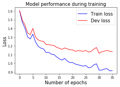這不會實例化變量 model = EmotionRecognitionCNN(num_classes=7, device=device, checkpoint_directory=checkpoint_directory) # 訓練模型 model.fit(training_data, eval_data, optimizer, num_epochs=500, early_stopping_rounds=5, verbose=10, train_from_scratch=False) ''' Train loss at epoch 1: 1.5994938561539342 Eval loss at epoch 1: 1.6061641948413006 Train loss at epoch 10: 1.1655063030448947 Eval loss at epoch 10: 1.2517835698296538 Train loss at epoch 20: 1.007327914901725 Eval loss at epoch 20: 1.1543473274306912 Train loss at epoch 30: 0.9942544895184863 Eval loss at epoch 30: 1.1808805191411382 ''' # 保存已訓練模型 model.save_model() ``` ## 在訓練期間展示表現 ```py pltplt..plotplot((rangerange((lenlen((modelmodel..historyhistory[['train_loss''train_l ])), model.history['train_loss'], color='b', label='Train loss'); plt.plot(range(len(model.history['eval_loss'])), model.history['eval_loss'], color='r', label='Dev loss'); plt.title('Model performance during training', fontsize=15) plt.xlabel('Number of epochs', fontsize=15); plt.ylabel('Loss', fontsize=15); plt.legend(fontsize=15); ```  ## 計算準確率 ```py train_acc = model.compute_accuracy(training_data) eval_acc = model.compute_accuracy(eval_data) print('Train accuracy: ', train_acc.result().numpy()) print('Eval accuracy: ', eval_acc.result().numpy()) ''' Train accuracy: 0.6615347103695706 Eval accuracy: 0.5728615213151296 ''' ``` ## 使用集成梯度展示神經網絡歸屬 所以現在我們已經訓練了我們的 CNN 模型，讓我們看看我們是否可以使用集成梯度來理解它的推理。本文詳細解釋了這種方法，稱為深度網絡的 Axiomatic 歸屬。 通常，你首先嘗試理解，模型的預測是直接計算輸出類對圖像的導數。這可以為你提供提示，圖像的哪個部分激活網絡。但是，這種技術對圖像偽影很敏感。 為了避免這種缺陷，我們將使用集成梯度來計算特定圖像的網絡歸屬。該技術簡單地采用原始圖像，將像素強度縮放到不同的度數（從`1/m`到`m`，其中`m`是步數）并且計算對每個縮放圖像的梯度。為了獲得該歸屬，對所有縮放圖像的梯度進行平均并與原始圖像相乘。 以下是使用 TensorFlow Eager 實現此操作的示例： ```py def get_prob_class(X, idx_class): """ 獲取所選圖像的 softmax 概率 Args: X: 4D tensor image. Returns: prob_class: the probability of the selected class. """ logits = model.predict(X, False) prob_class = logits[0, idx_class] return prob_class def integrated_gradients(X, m=200): """ 為一個圖像樣本計算集成梯度 Args: X: 4D tensor of the image sample. m: number of steps, more steps leads to a better approximation. Returns: g: integrated gradients. """ perc = (np.arange(1,m+1)/m).reshape(m,1,1,1) perc = tf.constant(perc, dtype=tf.float32) idx_class = tf.argmax(model.predict(X, False), axis=1).numpy()[0] X_tiled = tf.tile(X, [m,1,1,1]) X_scaled = tf.multiply(X_tiled, perc) grad_fn = tfe.gradients_function(get_prob_class, params=[0]) g = grad_fn(X_scaled, idx_class) g = tf.reduce_mean(g, axis=[1]) g = tf.multiply(X, g) return g, idx_class def visualize_attributions(X, g, idx_class): """ 使用集成漸變繪制原始圖像以及 CNN 歸屬。 Args: X: 4D tensor image. g: integrated gradients. idx_class: the index of the predicted label. """ img_attributions = X*tf.abs(g) f, (ax1, ax2) = plt.subplots(1, 2, sharey=True) ax1.imshow(X[0,:,:,0], cmap='gray') ax1.set_title('Predicted emotion: %s' %emotion_cat[idx_class], fontsize=15) ax2.imshow(img_attributions[0,:,:,0], cmap='gray') ax2.set_title('Integrated gradients', fontsize=15) plt.tight_layout() with tf.device(device): idx_img = 1000 # modify here to change the image X = tf.constant(X_train[idx_img,:].reshape(1,48,48,1)) g, idx_class = integrated_gradients(X, m=200) visualize_attributions(X, g, idx_class) ```  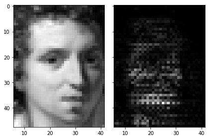集成梯度圖像的較亮部分對預測標簽的影響最大。 ## 網絡攝像頭測試 最后，你可以在任何新的圖像或視頻集上測試 CNN 的性能。 在下面的單元格中，我將向你展示如何使用網絡攝像頭捕獲圖像幀并對其進行預測。 為此，你必須安裝`opencv-python`庫。 你可以通過在終端輸入這些來輕松完成此操作： ``` pip install opencv-python ``` 正如你在筆記本開頭看到的那樣，FER2013 數據集中的圖像已經裁剪了面部。 為了裁剪新圖像/視頻中的人臉，我們將使用 OpenCV 庫中預先訓練的 Haar-Cascade 算法。 那么，讓我們開始吧！ 如果要在實時網絡攝像頭鏡頭上運行模型，請使用： ```py cap = cv2.VideoCapture(0) ``` 如果你有想要測試的預先錄制的視頻，可以使用： ```py cap = cv2.VideoCapture(path_video) ``` 自己隨意嘗試網絡！ 我保證這會很有趣。 ```py # 導入OpenCV import cv2 # 創建字符來將文本添加到圖像 font = cv2.FONT_HERSHEY_SIMPLEX # 導入與訓練的 Haar 級聯算法 face_cascade = cv2.CascadeClassifier(cv2.data.haarcascades + "haarcascade_frontalface_default.xml") ``` 網絡攝像頭捕獲的代碼受到[本教程](https://docs.opencv.org/3.0-beta/doc/py_tutorials/py_gui/py_video_display/py_video_display.html)的啟發。 ```py # Open video capture cap = cv2.VideoCapture(0) # Uncomment if you want to save the video along with its predictions # fourcc = cv2.VideoWriter_fourcc(*'mp4v') # out = cv2.VideoWriter('test_cnn.mp4', fourcc, 20.0, (720,480)) while(True): # 逐幀捕獲 ret, frame = cap.read() # 從 RGB 幀轉換為灰度 gray = cv2.cvtColor(frame, cv2.COLOR_BGR2GRAY) # 檢測幀中的所有人臉 faces = face_cascade.detectMultiScale(gray, 1.3, 5) # 遍歷發現的每個人臉 for (x,y,w,h) in faces: # 剪裁灰度幀中的人臉 face_gray = gray[y:y+h, x:x+w] # 將圖像大小改為 48x48 像素 face_res = cv2.resize(face_gray, (48,48)) face_res = face_res.reshape(1,48,48,1) # 按最大值標準化圖像 face_norm = face_res/255.0 # 模型上的正向傳播 with tf.device(device): X = tf.constant(face_norm) X = tf.cast(X, tf.float32) logits = model.predict(X, False) probs = tf.nn.softmax(logits) ordered_classes = np.argsort(probs[0])[::-1] ordered_probs = np.sort(probs[0])[::-1] k = 0 # 為每個預測繪制幀上的概率 for cl, prob in zip(ordered_classes, ordered_probs): # 添加矩形，寬度與其概率成比例 cv2.rectangle(frame, (20,100+k),(20+int(prob*100),130+k),(170,145,82),-1) # 向繪制的矩形添加表情標簽 cv2.putText(frame,emotion_cat[cl],(20,120+k),font,1,(0,0,0),1,cv2.LINE_AA) k += 40 # 如果你希望將視頻寫到磁盤，就取消注釋 #out.write(frame) # 展示所得幀 cv2.imshow('frame',frame) if cv2.waitKey(1) & 0xFF == ord('q'): break # 一切都完成后，解除捕獲 cap.release() cv2.destroyAllWindows() ```