# 十七、R 中的 TensorFlow 和 Keras R 是一個開源平臺，包括用于統計計算的環境和語言。它還有一個桌面和基于 Web 的 IDE，稱為 R Studio。有關 R 的更多信息，[請訪問此鏈接](https://www.r-project.org/)。 R 通過提供以下 R 包提供對 TensorFlow 和 Keras 的支持： * `tensorflow`包提供對 TF 核心 API 的支持 * `tfestimators`包提供對 TF 估計器 API 的支持 * `keras`包提供對 Keras API 的支持 * `tfruns`包用于 TensorBoard 風格的模型和訓練類可視化 在本章中，我們將學習如何在 R 中使用 TensorFlow，并將涵蓋以下主題： * 在 R 中安裝 TensorFlow 和 Keras 包 * R 中的 TF 核心 API * R 中的 TF 估計器 API * R 中的 Keras API * R 中的 TensorBoard * R 中的`tfruns`包 # 在 R 中安裝 TensorFlow 和 Keras 包 要在 R 中安裝支持 TensorFlow 和 Keras 的三個 R 包，請在 R 中執行以下命令。 1. 首先，安裝`devtools`： ```r install.packages("devtools") ``` 1. 安裝`tensorflow`和`tfestimators`包： ```r devtools::install_github("rstudio/tensorflow") devtools::install_github("rstudio/tfestimators") ``` 1. 加載`tensorflow`庫并安裝所需的功能： ```r library(tensorflow) install_tensorflow() ``` 1. 默認情況下，安裝功能會創建虛擬環境并在虛擬環境中安裝`tensorflow?`包。 有四種可用的安裝方法，可以使用`method`參數指定： | | | | --- | --- | | `auto` | 自動選擇當前平臺的默認值 | | `virtualenv` | 安裝到位于`~/.virtualenvs/r-tensorflow`的虛擬環境中 | | `conda` | 安裝到名為`r-tensorflow`的 Anaconda Python 環境中 | | `system` | 安裝到系統 Python 環境中 | 1. 默認情況下，安裝功能會安裝僅限 CPU 的 TensorFlow 版本。要安裝 GPU 版本，請使用版本參數： | | | | --- | --- | | `gpu` | 安裝`tensorflow-gpu` | | `nightly` | 安裝每晚 CPU 的版本 | | `nightly-gpu` | 安裝每晚 GPU 構建 | | `n.n.n` | 安裝特定版本，例如 1.3.0 | | `n.n.n-gpu` | 安裝特定版本的 GPU 版本，例如 1.3.0 | 如果您希望 TensorFlow 庫使用特定版本的 Python，請使用以下函數或設置`TENSORFLOW_PYTHON`環境變量： * `use_python('/usr/bin/python2')` * `use_virtualenv('~/venv')` * `use_condaenv('conda-env')` * `Sys.setenv(TENSORFLOW_PYTHON='/usr/bin/python2')` We installed TensorFLow in R on Ubuntu 16.04 using the following command: `install_tensorflow(version="gpu")? `Note that the installation does not support Python 3 at the time of writing this book. 1. 安裝 Keras 包： ```r devtools::install_github("rstudio/keras") ``` 1. 在虛擬環境中安裝 Keras： ```r library(keras) install_keras() ``` 1. 要安裝 GPU 版本，請使用： ```r install_keras(tensorflow = "gpu") ``` 1. 安裝`tfruns`包： ```r devtools::install_github("rstudio/tfruns") ``` # R 中的 TF 核心 API 我們在第 1 章中了解了 TensorFlow 核心 API。在 R 中，該 API 使用`tensorflow` R 包實現。 作為一個例子，我們提供了 MLP 模型的演練，[用于在此鏈接中對來自 MNIST 數據集的手寫數字進行分類](https://tensorflow.rstudio.com/tensorflow/articles/examples/mnist_softmax.html)。 您可以按照 Jupyter R 筆記本中的代碼`ch-17a_TFCore_in_R`。 1. 首先，加載庫： ```r library(tensorflow) ``` 1. 定義超參數： ```r batch_size <- 128 num_classes <- 10 steps <- 1000 ``` 1. 準備數據： ```r datasets <- tf$contrib$learn$datasets mnist <- datasets$mnist$read_data_sets("MNIST-data", one_hot = TRUE) ``` 數據從 TensorFlow 數據集庫加載，并已標準化為`[0, 1]`范圍。 1. 定義模型： ```r # Create the model x <- tf$placeholder(tf$float32, shape(NULL, 784L)) W <- tf$Variable(tf$zeros(shape(784L, num_classes))) b <- tf$Variable(tf$zeros(shape(num_classes))) y <- tf$nn$softmax(tf$matmul(x, W) + b) # Define loss and optimizer y_ <- tf$placeholder(tf$float32, shape(NULL, num_classes)) cross_entropy <- tf$reduce_mean(-tf$reduce_sum(y_ * log(y), reduction_indices=1L)) train_step <- tf$train$GradientDescentOptimizer(0.5)$minimize(cross_entropy) ``` 1. 訓練模型： ```r # Create session and initialize variables sess <- tf$Session() sess$run(tf$global_variables_initializer()) # Train for (i in 1:steps) { batches <- mnist$train$next_batch(batch_size) batch_xs <- batches[[1]] batch_ys <- batches[[2]] sess$run(train_step, feed_dict = dict(x = batch_xs, y_ = batch_ys)) } ``` 1. 評估模型： ```r correct_prediction <- tf$equal(tf$argmax(y, 1L), tf$argmax(y_, 1L)) accuracy <- tf$reduce_mean(tf$cast(correct_prediction, tf$float32)) score <-sess$run(accuracy, feed_dict = dict(x = mnist$test$images, y_ = mnist$test$labels)) cat('Test accuracy:', score, '\n') ``` 輸出如下： ```r Test accuracy: 0.9185 ``` 太酷了！ [通過此鏈接查找 R 中 TF 核心的更多示例](https://tensorflow.rstudio.com/tensorflow/articles/examples/)。 [有關`tensorflow` R 包的更多文檔可以在此鏈接中找到](https://tensorflow.rstudio.com/tensorflow/reference/)。 # R 中的 TF 估計器 API 我們在第 2 章中了解了 TensorFlow 估計器 API。在 R 中，此 API 使用`tfestimator` R 包實現。 例如，我們提供了 MLP 模型的演練，[用于在此鏈接中對來自 MNIST 數據集的手寫數字進行分類](https://tensorflow.rstudio.com/tfestimators/articles/examples/mnist.html)。 您可以按照 Jupyter R 筆記本中的代碼`ch-17b_TFE_Ttimator_in_R`。 1. 首先，加載庫： ```r library(tensorflow) library(tfestimators) ``` 1. 定義超參數： ```r batch_size <- 128 n_classes <- 10 n_steps <- 100 ``` 1. 準備數據： ```r # initialize data directory data_dir <- "~/datasets/mnist" dir.create(data_dir, recursive = TRUE, showWarnings = FALSE) # download the MNIST data sets, and read them into R sources <- list( train = list( x = "https://storage.googleapis.com/cvdf-datasets/mnist/train-images-idx3-ubyte.gz", y = "https://storage.googleapis.com/cvdf-datasets/mnist/train-labels-idx1-ubyte.gz" ), test = list( x = "https://storage.googleapis.com/cvdf-datasets/mnist/t10k-images-idx3-ubyte.gz", y = "https://storage.googleapis.com/cvdf-datasets/mnist/t10k-labels-idx1-ubyte.gz" ) ) # read an MNIST file (encoded in IDX format) read_idx <- function(file) { # create binary connection to file conn <- gzfile(file, open = "rb") on.exit(close(conn), add = TRUE) # read the magic number as sequence of 4 bytes magic <- readBin(conn, what="raw", n=4, endian="big") ndims <- as.integer(magic[[4]]) # read the dimensions (32-bit integers) dims <- readBin(conn,what="integer",n=ndims,endian="big") # read the rest in as a raw vector data <- readBin(conn,what="raw",n=prod(dims),endian="big") # convert to an integer vecto converted <- as.integer(data) # return plain vector for 1-dim array if (length(dims) == 1) return(converted) # wrap 3D data into matrix matrix(converted,nrow=dims[1],ncol=prod(dims[-1]),byrow=TRUE) } mnist <- rapply(sources,classes="character",how ="list",function(url) { # download + extract the file at the URL target <- file.path(data_dir, basename(url)) if (!file.exists(target)) download.file(url, target) # read the IDX file read_idx(target) }) # convert training data intensities to 0-1 range mnist$train$x <- mnist$train$x / 255 mnist$test$x <- mnist$test$x / 255 ``` 從下載的 gzip 文件中讀取數據，然后歸一化以落入`[0, 1]`范圍。 1. 定義模型： ```r # construct a linear classifier classifier <- linear_classifier( feature_columns = feature_columns( column_numeric("x", shape = shape(784L)) ), n_classes = n_classes # 10 digits ) # construct an input function generator mnist_input_fn <- function(data, ...) { input_fn( data, response = "y", features = "x", batch_size = batch_size, ... ) } ``` 1. 訓練模型： ```r train(classifier,input_fn=mnist_input_fn(mnist$train),steps=n_steps) ``` 1. 評估模型： ```r evaluate(classifier,input_fn=mnist_input_fn(mnist$test),steps=200) ``` 輸出如下： ```r Evaluation completed after 79 steps but 200 steps was specified ``` | average_loss | 損失 | global_step | 準確率 | | --- | --- | --- | --- | | 0.35656 | 45.13418 | 100 | 0.9057 | 太酷!! [通過此鏈接查找 R 中 TF 估計器的更多示例](https://tensorflow.rstudio.com/tfestimators/articles/examples/)。 [有關`tensorflow` R 包的更多文檔可以在此鏈接中找到](https://tensorflow.rstudio.com/tfestimators/reference/) # R 中的 Keras API 我們在第 3 章中了解了 Keras API。在 R 中，此 API 使用`keras` R 包實現。`keras` R 包實現了 Keras Python 接口的大部分功能，包括順序 API 和函數式 API。 作為示例，我們提供了 MLP 模型的演練，[用于在此鏈接中對來自 MNIST 數據集的手寫數字進行分類](https://keras.rstudio.com/articles/examples/mnist_mlp.html)。 您可以按照 Jupyter R 筆記本中的代碼`ch-17c_Keras_in_R`。 1. 首先，加載庫： ```r library(keras) ``` 1. 定義超參數： ```r batch_size <- 128 num_classes <- 10 epochs <- 30 ``` 1. 準備數據： ```r # The data, shuffled and split between train and test sets c(c(x_train, y_train), c(x_test, y_test)) %<-% dataset_mnist() x_train <- array_reshape(x_train, c(nrow(x_train), 784)) x_test <- array_reshape(x_test, c(nrow(x_test), 784)) # Transform RGB values into [0,1] range x_train <- x_train / 255 x_test <- x_test / 255 cat(nrow(x_train), 'train samples\n') cat(nrow(x_test), 'test samples\n') # Convert class vectors to binary class matrices y_train <- to_categorical(y_train, num_classes) y_test <- to_categorical(y_test, num_classes) ``` 注釋是不言自明的：數據從 Keras 數據集庫加載，然后轉換為 2D 數組并歸一化為`[0, 1]`范圍。 1. 定義模型： ```r model <- keras_model_sequential() model %>% layer_dense(units=256,activation='relu',input_shape=c(784)) %>% layer_dropout(rate = 0.4) %>% layer_dense(units = 128, activation = 'relu') %>% layer_dropout(rate = 0.3) %>% layer_dense(units = 10, activation = 'softmax') summary(model) model %>% compile( loss = 'categorical_crossentropy', optimizer = optimizer_rmsprop(), metrics = c('accuracy') ) ``` 1. 定義和編譯順序模型。我們得到的模型定義如下： ```r _____________________________________________________ Layer (type) Output Shape Param # ===================================================== dense_26 (Dense) (None, 256) 200960 _____________________________________________________ dropout_14 (Dropout) (None, 256) 0 _____________________________________________________ dense_27 (Dense) (None, 128) 32896 _____________________________________________________ dropout_15 (Dropout) (None, 128) 0 _____________________________________________________ dense_28 (Dense) (None, 10) 1290 ===================================================== Total params: 235,146 Trainable params: 235,146 Non-trainable params: 0 ``` 1. 訓練模型： ```r history <- model %>% fit( x_train, y_train, batch_size = batch_size, epochs = epochs, verbose = 1, validation_split = 0.2 ) plot(history) ``` 擬合函數的輸出存儲在歷史對象中，其包含來自訓練周期的損失和度量值。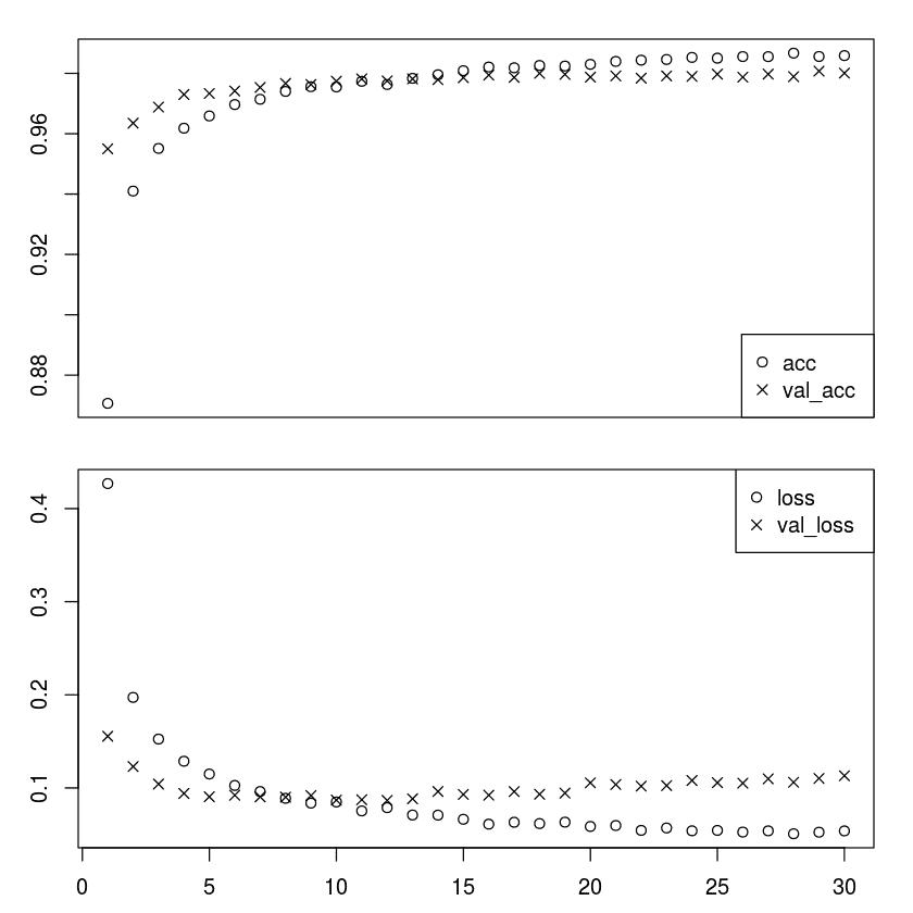繪制歷史對象中的數據，結果如下： Training and Validation Accuracy (y-axis) in Epochs (x-axis) 1. 評估模型： ```r score <- model %>% evaluate( x_test, y_test, verbose = 0 ) # Output metrics cat('Test loss:', score[[1]], '\n') cat('Test accuracy:', score[[2]], '\n') ``` 輸出如下： ```r Test loss: 0.1128517 Test accuracy: 0.9816 ``` 太酷!! [在此鏈接中查找更多關于 R 中的 Keras 的示例](https://keras.rstudio.com/articles/examples/index.html)。 [有關 Keras R 包的更多文檔可在此鏈接中找到](https://keras.rstudio.com/reference/index.html)。 # R 中的 TensorBoard 您可以按照 Jupyter R 筆記本中的代碼`ch-17d_TensorBoard_in_R`。 您可以使用`tensorboard()`函數查看 TensorBoard，如下所示： ```r tensorboard('logs') ``` 這里，`'logs'`是應該創建 TensorBoard 日志的文件夾。 數據將顯示為執行周期并記錄數據。在 R 中，收集 TensorBoard 的數據取決于所使用的包： * 如果您使用的是`tensorflow`包，請將`tf$summary$scalar`操作附加到圖中 * 如果您使用的是`tfestimators`包，則 TensorBoard 數據會自動寫入創建估計器時指定的`model_dir`參數 * 如果您正在使用`keras`包，則必須在使用`fit()`函數訓練模型時包含`callback_tensorboard()`函數 我們修改了之前提供的 Keras 示例中的訓練，如下所示： ```r # Training the model -------- tensorboard("logs") history <- model %>% fit( x_train, y_train, batch_size = batch_size, epochs = epochs, verbose = 1, validation_split = 0.2, callbacks = callback_tensorboard("logs") ) ``` 當我們執行筆記本時，我們獲得了訓練單元的以下輸出： ```r Started TensorBoard at http://127.0.0.1:4233 ``` 當我們點擊鏈接時，我們會看到在 TensorBoard 中繪制的標量： 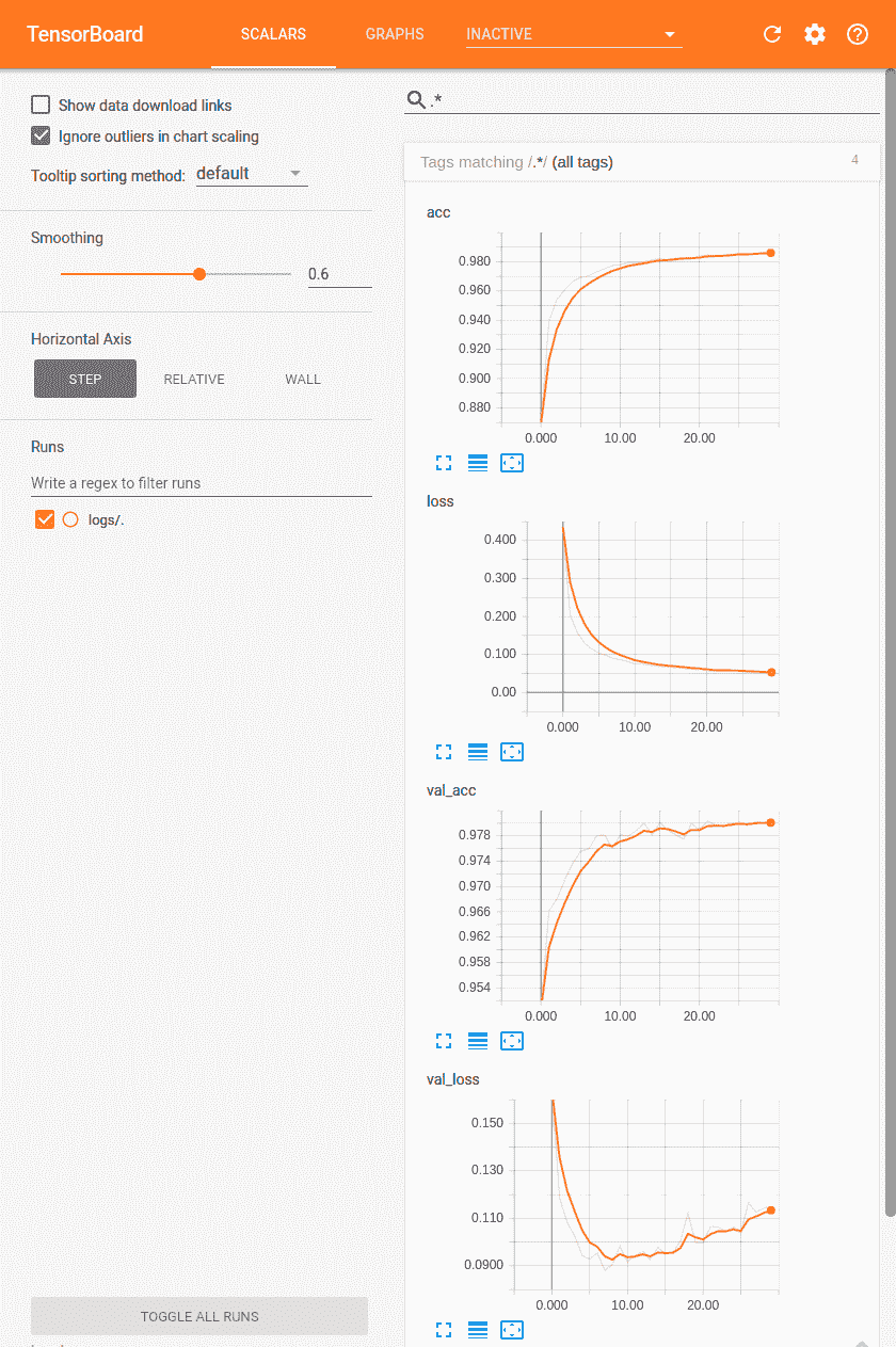TensorBoad Visualization of Plots 單擊 Graphs 選項卡，我們在 TensorBoard 中看到計算圖：  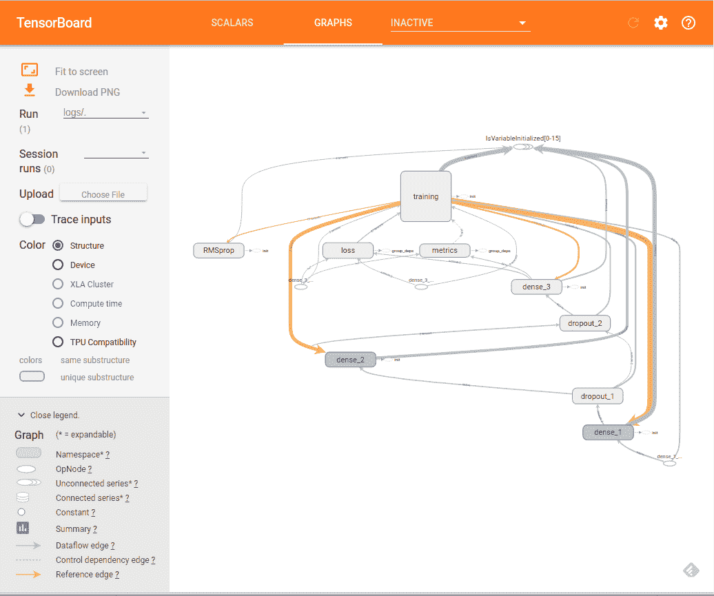TensorBoard 計算圖的可視化有關 R 中 TensorBoard 的更多文檔，[請訪問此鏈接](https://tensorflow.rstudio.com/tools/tensorboard.html)。 # R 中的`tfruns`包 您可以按照 Jupyter R 筆記本中的代碼`ch-17d_TensorBoard_in_R`。 `tfruns`包是 R 中提供的非常有用的工具，有助于跟蹤多次運行以訓練模型。對于使用`keras` `tfestimators`包在 R 中構建的模型，`tfruns`包自動捕獲運行數據。使用`tfruns`非常簡單易行。只需在 R 文件中創建代碼，然后使用`training_run()`函數執行該文件。例如，如果你有一個`mnist_model.R?`文件 ，那么在交互式 R 控制臺中使用`training_run()`函數執行它，如下所示： ```r library(tfruns) training_run('mnist_model.R') ``` 訓練完成后，將自動顯示顯示運行摘要的窗口。我們從[`tfruns` GitHub 倉庫](https://github.com/rstudio/tfruns/blob/master/inst/examples/mnist_mlp/mnist_mlp)獲得的[`mnist_mlp.R`](https://github.com/rstudio/tfruns/blob/master/inst/examples/mnist_mlp/mnist_mlp.R)窗口中獲得以下輸出。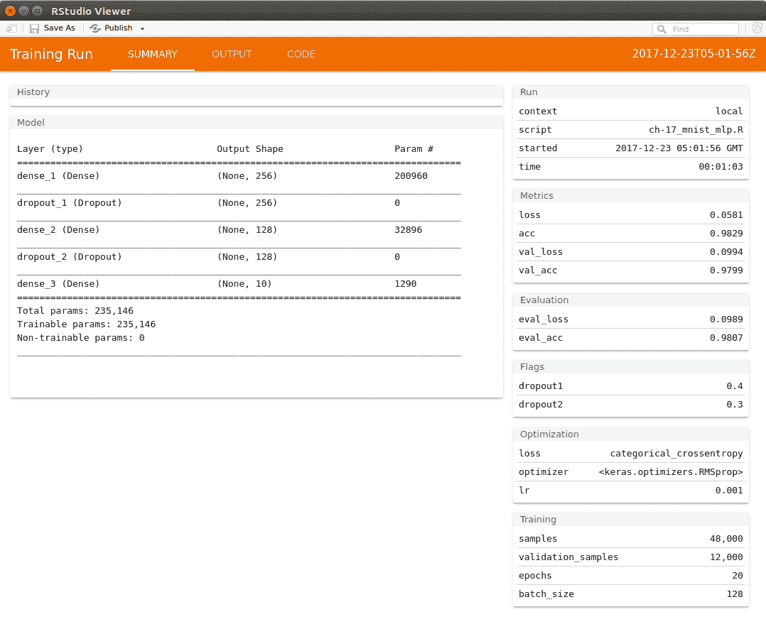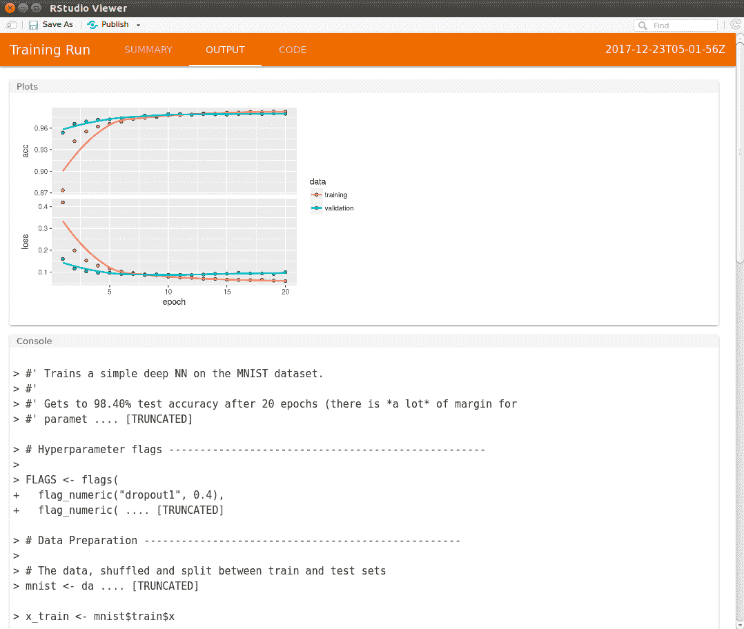 tfruns visualization of the model run 在“查看器”窗口中，輸出選項卡包含以下圖： tfruns visualization of the accuracy and loss values `tfruns`包將一個插件安裝到 RStudio，也可以從`Addins`菜單選項訪問。該包還允許您比較多個運行并將運行報告發布到 RPub 或 RStudio Connect。您還可以選擇在本地保存報告。 有關 R 中`tfruns`包的更多文檔，請訪問以下鏈接： <https://tensorflow.rstudio.com/tools/tfruns/reference/> <https://tensorflow.rstudio.com/tools/tfruns/articles/overview.html>. # 總結 在本章中，我們學習了如何在 R 中使用 TensorFlow 核心，TensorFlow 估計器和 Keras 包來構建和訓練機器學習模型。我們提供了來自 RStudio 的 MNIST 示例的演練，并提供了有關 TensorFlow 和 Keras R 包的進一步文檔的鏈接。我們還學習了如何使用 R 中的可視化工具 TensorBoard。我們還介紹了一個來自 R Studio 的新工具`tfruns`，它允許您為多次運行創建報告，分析和比較它們，并在本地保存或發布它們。 直接在 R 中工作的能力很有用，因為大量的生產數據科學和機器學習代碼是使用 R 編寫的，現在您可以將 TensorFlow 集成到相同的代碼庫中并在 R 環境中運行它。 在下一章中，我們將學習一些用于調試構建和訓練 TensorFlow 模型的代碼的技術。