四、TensorFlow 2 和監督機器學習 · ApacheCN 深度學習譯文集

# 四、TensorFlow 2 和監督機器學習在本章中，我們將討論并舉例說明 TensorFlow 2 在以下情況下的監督機器學習問題中的使用：線性回歸，邏輯回歸和 **K 最近鄰**（**KNN**）。在本章中，我們將研究以下主題： * 監督學習 * 線性回歸 * 我們的第一個線性回歸示例 * 波士頓住房數據集 * 邏輯回歸（分類） * **K 最近鄰**（**KNN**） # 監督學習監督學習是一種機器學習場景，其中一組數據點中的一個或多個數據點與標簽關聯。然后，模型*學習*，以預測看不見的數據點的標簽。為了我們的目的，每個數據點通常都是張量，并與一個標簽關聯。在計算機視覺中，有很多受監督的學習問題；例如，算法顯示了許多成熟和未成熟的西紅柿的圖片，以及表明它們是否成熟的分類標簽，并且在訓練結束后，該模型能夠根據訓練集預測未成熟的西紅柿的狀態。這可能在番茄的物理分揀機制中有非常直接的應用。或一種算法，該算法可以在顯示許多示例以及它們的性別和年齡之后，學會預測新面孔的性別和年齡。此外，如果模型已經在許多樹圖像及其類型標簽上進行了訓練，則可以學習根據樹圖像來預測樹的類型可能是有益的。 # 線性回歸線性回歸問題是在給定一個或多個其他變量（數據點）的值的情況下，您必須預測一個*連續*變量的值的問題。例如，根據房屋的占地面積，預測房屋的售價。在這些示例中，您可以將已知特征及其關聯的標簽繪制在簡單的線性圖上，如熟悉的`x, y`散點圖，并繪制最適合數據的線。這就是最適合的**系列**。然后，您可以讀取對應于該圖的`x`范圍內的任何特征值的標簽。但是，線性回歸問題可能涉及幾個特征，其中使用了術語**多個**或**多元線性回歸**。在這種情況下，不是最適合數據的線，而是一個平面（兩個特征）或一個超平面（兩個以上特征）。在房價示例中，我們可以將房間數量和花園的長度添加到特征中。有一個著名的數據集，稱為波士頓住房數據集，[涉及 13 個特征](https://www.kaggle.com/c/ml210-boston)。考慮到這 13 個特征，此處的回歸問題是預測波士頓郊區的房屋中位數。術語：特征也稱為預測變量或自變量。標簽也稱為響應變量或因變量。 # 我們的第一個線性回歸示例我們將從一個簡單的，人為的，線性回歸問題開始設置場景。在此問題中，我們構建了一個人工數據集，首先在其中創建，因此知道了我們要擬合的線，但是隨后我們將使用 TensorFlow 查找這條線。我們執行以下操作-在導入和初始化之后，我們進入一個循環。在此循環內，我們計算總損失（定義為點的數據集`y`的均方誤差）。然后，我們根據我們的權重和偏置來得出這種損失的導數。這將產生可用于調整權重和偏差以降低損失的值；這就是所謂的梯度下降。通過多次重復此循環（技術上稱為**周期**），我們可以將損失降低到盡可能低的程度，并且可以使用訓練有素的模型進行預測。首先，我們導入所需的模塊（回想一下，急切執行是默認的）： ```py import tensorflow as tf import numpy as np ``` 接下來，我們初始化重要的常量，如下所示： ```py n_examples = 1000 # number of training examples training_steps = 1000 # number of steps we are going to train for display_step = 100 # after multiples of this, we display the loss learning_rate = 0.01 # multiplying factor on gradients m, c = 6, -5 # gradient and y-intercept of our line, edit these for a different linear problem ``` 給定`weight`和`bias`（`m`和`c`）的函數，用于計算預測的`y`： ```py def train_data(n, m, c): x = tf.random.normal([n]) # n values taken from a normal distribution, noise = tf.random.normal([n])# n values taken from a normal distribution y = m*x + c + noise # our scatter plot return x, y def prediction(x, weight, bias): return weight*x + bias # our predicted (learned) m and c, expression is like y = m*x + c ``` 用于獲取初始或預測的權重和偏差并根據`y`計算均方損失（偏差）的函數： ```py def loss(x, y, weights, biases): error = prediction(x, weights, biases) - y # how 'wrong' our predicted (learned) y is squared_error = tf.square(error) return tf.reduce_mean(input_tensor=squared_error) # overall mean of squared error, scalar value. ``` 這就是 TensorFlow 發揮作用的地方。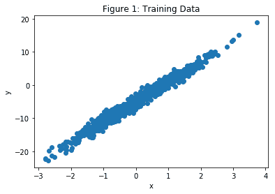使用名為`GradientTape()`的類，我們可以編寫一個函數來計算相對于`weights`和`bias`的損失的導數（梯度）： ```py def grad(x, y, weights, biases): with tf.GradientTape() as tape: loss_ = loss(x, y, weights, biases) return tape.gradient(loss, [weights, bias]) # direction and value of the gradient of our weights and biases ``` 為訓練循環設置回歸器，并顯示初始損失，如下所示： ```py x, y = train_data(n_examples,m,c) # our training values x and y plt.scatter(x,y) plt.xlabel("x") plt.ylabel("y") plt.title("Figure 1: Training Data") W = tf.Variable(np.random.randn()) # initial, random, value for predicted weight (m) B = tf.Variable(np.random.randn()) # initial, random, value for predicted bias (c) print("Initial loss: {:.3f}".format(loss(x, y, W, B))) ``` 輸出如下所示： ![](https://img.kancloud.cn/61/7b/617b819698fc5ebceeabb6d9546e7654_394x278.png) 接下來，我們的主要訓練循環。這里的想法是根據我們的`learning_rate`來少量調整`weights`和`bias`，以將損失依次降低到我們最適合的線上收斂的點： ```py for step in range(training_steps): #iterate for each training step deltaW, deltaB = grad(x, y, W, B) # direction(sign) and value of the gradients of our loss # with respect to our weights and bias change_W = deltaW * learning_rate # adjustment amount for weight change_B = deltaB * learning_rate # adjustment amount for bias W.assign_sub(change_W) # subract change_W from W B.assign_sub(change_B) # subract change_B from B if step==0 or step % display_step == 0: # print(deltaW.numpy(), deltaB.numpy()) # uncomment if you want to see the gradients print("Loss at step {:02d}: {:.6f}".format(step, loss(x, y, W, B))) ``` 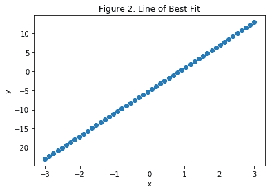最終結果如下： ```py print("Final loss: {:.3f}".format(loss(x, y, W, B))) print("W = {}, B = {}".format(W.numpy(), B.numpy())) print("Compared with m = {:.3f}, c = {:.3f}".format(m, c)," of the original line") xs = np.linspace(-3, 4, 50) ys = W.numpy()*xs + B.numpy() plt.scatter(xs,ys) plt.xlabel("x") plt.ylabel("y") plt.title("Figure 2: Line of Best Fit") ``` 您應該看到，發現`W`和`B`的值非常接近我們用于`m`和`c`的值，這是可以預期的： ![](https://img.kancloud.cn/74/47/7447d03814205745bcbedb5591d7e606_394x278.png) # 波士頓住房數據集接下來，我們將類似的回歸技術應用于波士頓房屋數據集。此模型與我們之前的僅具有一個特征的人工數據集之間的主要區別在于，波士頓房屋數據集是真實數據，具有 13 個特征。這是一個回歸問題，因為我們認為房價（即標簽）被不斷估價。同樣，我們從導入開始，如下所示： ```py import tensorflow as tf from sklearn.datasets import load_boston from sklearn.preprocessing import scale import numpy as np ``` 我們的重要常數如下所示： ```py learning_rate = 0.01 epochs = 10000 display_epoch = epochs//20 n_train = 300 n_valid = 100 ``` 接下來，我們加載數據集并將其分為訓練，驗證和測試集。我們在訓練集上進行訓練，并在驗證集上檢查和微調我們的訓練模型，以確保例如沒有過擬合。然后，我們使用測試集進行最終精度測量，并查看我們的模型在完全看不見的數據上的表現如何。注意`scale`方法。這用于將數據轉換為均值為零且單位標準差為零的集合。 `sklearn.preprocessing`方法`scale`通過從特征集中的每個數據點減去平均值，然后將每個特征除以該特征集的標準差來實現此目的。這樣做是因為它有助于我們模型的收斂。所有特征也都轉換為`float32`數據類型： ```py features, prices = load_boston(True) n_test = len(features) - n_train - n_valid # Keep n_train samples for training train_features = tf.cast(scale(features[:n_train]), dtype=tf.float32) train_prices = prices[:n_train] # Keep n_valid samples for validation valid_features = tf.cast(scale(features[n_train:n_train+n_valid]), dtype=tf.float32) valid_prices = prices[n_train:n_train+n_valid] # Keep remaining n_test data points as test set) test_features = tf.cast(scale(features[n_train+n_valid:n_train+n_valid+n_test]), dtype=tf.float32) test_prices = prices[n_train + n_valid : n_train + n_valid + n_test] ``` 接下來，我們具有與上一個示例相似的函數。首先，請注意我們現在使用的是更流行的路徑，均方誤差： ```py # A loss function using root mean-squared error def loss(x, y, weights, bias): error = prediction(x, weights, bias) - y # how 'wrong' our predicted (learned) y is squared_error = tf.square(error) return tf.sqrt(tf.reduce_mean(input_tensor=squared_error)) # squre root of overall mean of squared error. ``` 接下來，我們找到相對于`weights`和`bias`的損失梯度的方向和值： ```py # Find the derivative of loss with respect to weight and bias def gradient(x, y, weights, bias): with tf.GradientTape() as tape: loss_value = loss(x, y, weights, bias) return tape.gradient(loss_value, [weights, bias])# direction and value of the gradient of our weight and bias ``` 然后，我們查詢設備，將初始權重設置為隨機值，將`bias`設置為`0`，然后打印初始損失。請注意，`W`現在是`1`向量的`13`，如下所示： ```py # Start with random values for W and B on the same batch of data W = tf.Variable(tf.random.normal([13, 1],mean=0.0, stddev=1.0, dtype=tf.float32)) B = tf.Variable(tf.zeros(1) , dtype = tf.float32) print(W,B) print("Initial loss: {:.3f}".format(loss(train_features, train_prices,W, B))) ``` 現在，進入我們的主要訓練循環。這里的想法是根據我們的`learning_rate`將`weights`和`bias`進行少量調整，以將損失逐步降低至我們已經收斂到最佳擬合線的程度。如前所述，此技術稱為**梯度下降**： ```py for e in range(epochs): #iterate for each training epoch deltaW, deltaB = gradient(train_features, train_prices, W, B) # direction (sign) and value of the gradient of our weight and bias change_W = deltaW * learning_rate # adjustment amount for weight change_B = deltaB * learning_rate # adjustment amount for bias W.assign_sub(change_W) # subract from W B.assign_sub(change_B) # subract from B if e==0 or e % display_epoch == 0: # print(deltaW.numpy(), deltaB.numpy()) # uncomment if you want to see the gradients print("Validation loss after epoch {:02d}: {:.3f}".format(e, loss(valid_features, valid_prices, W, B))) ``` 最后，讓我們將實際房價與其預測值進行比較，如下所示： ```py example_house = 69 y = test_prices[example_house] y_pred = prediction(test_features,W.numpy(),B.numpy())[example_house] print("Actual median house value",y," in $10K") print("Predicted median house value ",y_pred.numpy()," in $10K") ``` # 邏輯回歸（分類）這類問題的名稱令人迷惑，因為正如我們所看到的，回歸意味著連續值標簽，例如房屋的中位數價格或樹的高度。邏輯回歸并非如此。當您遇到需要邏輯回歸的問題時，這意味著標簽為`categorical`；例如，零或一，`True`或`False`，是或否，貓或狗，或者它可以是兩個以上的分類值；例如，紅色，藍色或綠色，或一，二，三，四或五，或給定花的類型。標簽通常具有與之相關的概率；例如，`P(cat = 0.92)`，`P(dog = 0.08)`。因此，邏輯回歸也稱為**分類**。在下一個示例中，我們將使用`fashion_mnist`數據集使用邏輯回歸來預測時尚商品的類別。這里有一些例子： ![](https://img.kancloud.cn/a9/48/a9489005f365ce15d15c7633c673ce23_959x113.png) 邏輯回歸以預測項目類別我們可以在 50,000 張圖像上訓練模型，在 10,000 張圖像上進行驗證，并在另外 10,000 張圖像上進行測試。首先，我們導入建立初始模型和對其進行訓練所需的模塊，并啟用急切的執行： ```py import numpy as np import tensorflow as tf import keras from tensorflow.python.keras.datasets import fashion_mnist #this is our dataset from keras.callbacks import ModelCheckpoint tf.enable_eager_execution() ``` 接下來，我們初始化重要的常量，如下所示： ```py # important constants batch_size = 128 epochs = 20 n_classes = 10 learning_rate = 0.1 width = 28 # of our images height = 28 # of our images ``` 然后，我們將我們訓練的時尚標簽的`indices`與它們的標簽相關聯，以便稍后以圖形方式打印出結果： ```py fashion_labels = ["Shirt/top","Trousers","Pullover","Dress","Coat","Sandal","Shirt","Sneaker","Bag","Ankle boot"] #indices 0 1 2 3 4 5 6 7 8 9 # Next, we load our fashion data set, # load the dataset (x_train, y_train), (x_test, y_test) = fashion_mnist.load_data() ``` 然后，我們將每個圖像中的每個整數值像素轉換為`float32`并除以 255 以對其進行歸一化： ```py # normalize the features for better training x_train = x_train.astype('float32') / 255. x_test = x_test.astype('float32') / 255. ``` `x_train`現在由`60000`，`float32`值組成，并且`x_test`保持`10000`相似的值。然后，我們展平特征集，準備進行訓練： ```py # flatten the feature set for use by the training algorithm x_train = x_train.reshape((60000, width * height)) x_test = x_test.reshape((10000, width * height)) ``` 然后，我們將訓練集`x_train`和`y_train`進一步分為訓練集和驗證集： ```py split = 50000 #split training sets into training and validation sets (x_train, x_valid) = x_train[:split], x_train[split:] (y_train, y_valid) = y_train[:split], y_train[split:] ``` 如果標簽是單熱編碼的，那么許多機器學習算法效果最好，因此我們接下來要做。但請注意，我們會將產生的一束熱張量轉換回（單熱）NumPy 數組，以備稍后由 Keras 使用： ```py # one hot encode the labels using TensorFLow. # then convert back to numpy as we cannot combine numpy # and tensors as input to keras later y_train_ohe = tf.one_hot(y_train, depth=n_classes).numpy() y_valid_ohe = tf.one_hot(y_valid, depth=n_classes).numpy() y_test_ohe = tf.one_hot(y_test, depth=n_classes).numpy() #or use tf.keras.utils.to_categorical(y_train,10) ``` 這是一段代碼，其中顯示了一個介于零到九之間的值以及其單熱編碼版本： ```py # show difference between original label and one-hot-encoded label i=5 print(y_train[i]) # 'ordinairy' number value of label at index i print (tf.one_hot(y_train[i], depth=n_classes))# same value as a 1\. in correct position in an length 10 1D tensor print(y_train_ohe[i]) # same value as a 1\. 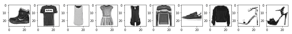in correct position in an length 10 1D numpy array ``` 在這里重要的是要注意索引`i`和存儲在索引`i`的標簽之間的差異。這是另一段代碼，顯示`y_train`中的前 10 個時尚項目： ```py # print sample fashion images. # we have to reshape the image held in x_train back to width by height # as we flattened it for training into width*height import matplotlib.pyplot as plt %matplotlib inline _,image = plt.subplots(1,10,figsize=(8,1)) for i in range(10): image[i].imshow(np.reshape(x_train[i],(width, height)), cmap="Greys") print(fashion_labels[y_train[i]],sep='', end='') ``` 現在，我們進入代碼的重要且可概括的部分。 Google 建議，對于創建任何類型的機器學習模型，都可以通過將其分類為`tf.keras.Model`來創建模型。這具有直接的優勢，即我們可以在我們的子類化模型中使用`tf.keras.Model`的所有功能，包括編譯和訓練例程以及層功能，在后續的章節中，我們將詳細介紹。對于我們的邏輯回歸示例，我們需要在子類中編寫兩個方法。首先，我們需要編寫一個構造器，該構造器調用超類的構造器，以便正確創建模型。在這里，我們傳入正在使用的類數（`10`），并在實例化模型以創建單個層時使用此構造器。我們還必須聲明`call`方法，并使用該方法來編程在模型訓練的正向傳遞過程中發生的情況。稍后，當我們考慮具有前向和后向傳遞的神經網絡時，我們將對這種情況進行更多說明。對于我們當前的目的，我們只需要知道在`call`方法中，我們采用輸入的`softmax`來產生輸出。 `softmax`函數的作用是獲取一個向量（或張量），然后在其元素具有該向量最大值的位置上用幾乎為 1 的值覆蓋，在所有其他位置上使用幾乎為零的值覆蓋。這與單熱編碼很相似。請注意，在此方法中，由于`softmax`未為 GPU 實現，因此我們必須在 CPU 上強制執行： ```py # model definition (the canonical Google way) class LogisticRegression(tf.keras.Model): def __init__(self, num_classes): super(LogisticRegression, self).__init__() # call the constructor of the parent class (Model) self.dense = tf.keras.layers.Dense(num_classes) #create an empty layer called dense with 10 elements. def call(self, inputs, training=None, mask=None): # required for our forward pass output = self.dense(inputs) # copy training inputs into our layer # softmax op does not exist on the gpu, so force execution on the CPU with tf.device('/cpu:0'): output = tf.nn.softmax(output) # softmax is near one for maximum value in output # and near zero for the other values. return output ``` 現在，我們準備編譯和訓練我們的模型。首先，我們確定可用的設備，然后使用它。然后，使用我們開發的類聲明模型。聲明要使用的優化程序后，我們將編譯模型。我們使用的損失，分類交叉熵（也稱為**對數損失**），通常用于邏輯回歸，因為要求預測是概率。優化器是一個選擇和有效性的問題，[有很多可用的方法](https://www.tensorflow.org/api_guides/python/train#Optimizers)。接下來是帶有三個參數的`model.compile`調用。我們將很快看到，它為我們的訓練模型做準備。在撰寫本文時，優化器的選擇是有限的。 `categorical_crossentropy`是多標簽邏輯回歸問題的正態損失函數，`'accuracy'`度量是通常用于分類問題的度量。請注意，接下來，我們必須使用樣本大小僅為輸入圖像之一的`model.call`方法進行虛擬調用，否則`model.fit`調用將嘗試將整個數據集加載到內存中以確定輸入特征的大小。接下來，我們建立一個`ModelCheckpoint`實例，該實例用于保存訓練期間的最佳模型，然后使用`model.fit`調用訓練模型。找出`model.compile`和`model.fit`（以及所有其他 Python 或 TensorFlow 類或方法）的所有不同參數的最簡單方法是在 Jupyter 筆記本中工作，然后按`Shift + TAB + TAB`，當光標位于相關類或方法調用上時。從代碼中可以看到，`model.fit`在訓練時使用`callbacks`方法（由驗證準確率確定）保存最佳模型，然后加載最佳模型。最后，我們在測試集上評估模型，如下所示： ```py # build the model model = LogisticRegression(n_classes) # compile the model #optimiser = tf.train.GradientDescentOptimizer(learning_rate) optimiser =tf.keras.optimizers.Adam() #not supported in eager execution mode. model.compile(optimizer=optimiser, loss='categorical_crossentropy', metrics=['accuracy'], ) # TF Keras tries to use the entire dataset to determine the shape without this step when using .fit() # So, use one sample of the provided input dataset size to determine input/output shapes for the model dummy_x = tf.zeros((1, width * height)) model.call(dummy_x) checkpointer = ModelCheckpoint(filepath="./model.weights.best.hdf5", verbose=2, save_best_only=True, save_weights_only=True) # train the model model.fit(x_train, y_train_ohe, batch_size=batch_size, epochs=epochs, validation_data=(x_valid, y_valid_ohe), callbacks=[checkpointer], verbose=2) #load model with the best validation accuracy model.load_weights("./model.weights.best.hdf5") # evaluate the model on the test set scores = model.evaluate(x_test, y_test_ohe, batch_size, verbose=2) print("Final test loss and accuracy :", scores) y_predictions = model.predict(x_test) ``` 最后，對于我們的邏輯回歸示例，我們有一些代碼可以檢查一個時尚的測試項目，以查看其預測是否準確： ```py # example of one predicted versus one true fashion label index = 42 index_predicted = np.argmax(y_predictions[index]) # largest label probability index_true = np.argmax(y_test_ohe[index]) # pick out index of element with a 1 in it print("When prediction is ",index_predicted) print("ie. predicted label is", fashion_labels[index_predicted]) print("True label is ",fashion_labels[index_true]) print ("\n\nPredicted V (True) fashion labels, green is correct, red is wrong") size = 12 # i.e. 12 random numbers chosen out of x_test.shape[0] =1000, we do not replace them fig = plt.figure(figsize=(15,3)) rows = 3 cols = 4 ``` 檢查 12 個預測的隨機樣本，如下所示： ```py for i, index in enumerate(np.random.choice(x_test.shape[0], size = size, replace = False)): axis = fig.add_subplot(rows,cols,i+1, xticks=[], yticks=[]) # position i+1 in grid with rows rows and cols columns axis.imshow(x_test[index].reshape(width,height), cmap="Greys") index_predicted = np.argmax(y_predictions[index]) index_true = np.argmax(y_test_ohe[index]) axis.set_title(("{} ({})").format(fashion_labels[index_predicted],fashion_labels[index_true]), color=("green" if index_predicted==index_true else "red")) ``` 以下屏幕快照顯示了真實與（預測）時尚標簽： ![](https://img.kancloud.cn/e0/11/e0117b3594681fb921fbe40106121360_747x486.png) 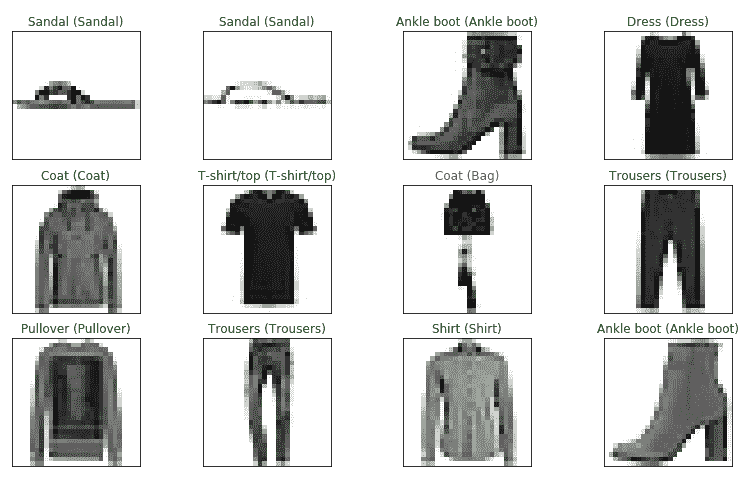時尚標簽到此結束我們對邏輯回歸的研究。現在，我們將看看另一種非常強大的監督學習技術，即 K 最近鄰。 # K 最近鄰（KNN） KNN 背后的想法相對簡單。給定新的特定數據點的值，請查看該點的 KNN，并根據該 k 個鄰居的標簽為該點分配標簽，其中`k`是算法的參數。在這種情況下，沒有這樣構造的模型。該算法僅查看數據集中新點與所有其他數據點之間的所有距離，接下來，我們將使用由三種類型的鳶尾花組成的著名數據集：`iris setosa`， `iris virginica`和`iris versicolor`。對于這些標簽中的每一個，特征都是花瓣長度，花瓣寬度，萼片長度和萼片寬度。有關顯示此數據集的圖表，請參見[這里](https://en.wikipedia.org/wiki/Iris_flower_data_set#/media/File:Iris_dataset_scatterplot.svg)。有 150 個數據點（每個數據點都包含前面提到的四個測量值）和 150 個相關標簽。我們將它們分為 120 個訓練數據點和 30 個測試數據點。首先，我們有通常的導入，如下所示： ```py import numpy as np from sklearn import datasets import tensorflow as tf # and we next load our data: iris = datasets.load_iris() x = np.array([i for i in iris.data]) y = np.array(iris.target) x.shape, y.shape ``` 然后，我們將花標簽放在列表中以備后用，如下所示： ```py flower_labels = ["iris setosa", "iris virginica", "iris versicolor"] ``` 現在是時候對標簽進行一次熱編碼了。 `np.eye`返回一個二維數組，在對角線上有一個，默認為主對角線。然后用`y`進行索引為我們提供了所需的`y`單熱編碼： ```py #one hot encoding, another method y = np.eye(len(set(y)))[y] y[0:10] ``` 接下來，我們將特征規格化為零到一，如下所示： ```py x = (x - x.min(axis=0)) / (x.max(axis=0) - x.min(axis=0)) ``` 為了使算法正常工作，我們必須使用一組隨機的訓練特征。接下來，我們還要通過從數據集的整個范圍中刪除訓練指標來設置測試指標： ```py # create indices for the train-test split np.random.seed(42) split = 0.8 # this makes 120 train and 30 test features train_indices = np.random.choice(len(x), round(len(x) * split), replace=False) test_indices =np.array(list(set(range(len(x))) - set(train_indices))) ``` 我們現在可以創建我們的訓練和測試特征，以及它們的相關標簽： ```py # the train-test split train_x = x[train_indices] test_x = x[test_indices] train_y = y[train_indices] test_y = y[test_indices] ``` 現在，我們將`k`的值設置為`5`，如下所示： ```py k = 5 ``` 接下來，在 Jupyter 筆記本中，我們具有預測測試數據點類別的函數。我們將逐行對此進行細分。首先是我們的`distance`函數。執行此函數后，可變距離包含我們 120 個訓練點與 30 個測試點之間的所有（曼哈頓）距離；也就是說，由 30 行乘 120 列組成的數組-曼哈頓距離，有時也稱為**城市街區距離**，是`x[1], x[2]`的兩個數據點向量的值之差的絕對值；即`|x[1] - x[2]|`。如果需要的話（如本例所示），將使用各個特征差異的總和。 `tf.expand`在`test_x`上增加了一個額外的維數，以便在減法發生之前，可以通過廣播使兩個數組*擴展*以使其與減法兼容。由于`x`具有四個特征，并且`reduce_sum`超過`axis=2`，因此結果是我們 30 個測試點和 120 個訓練點之間的距離的 30 行。所以我們的`prediction`函數是： ```py def prediction(train_x, test_x, train_y,k): print(test_x) d0 = tf.expand_dims(test_x, axis =1) d1 = tf.subtract(train_x, d0) d2 = tf.abs(d1) distances = tf.reduce_sum(input_tensor=d2, axis=2) print(distances) # or # distances = tf.reduce_sum(tf.abs(tf.subtract(train_x, tf.expand_dims(test_x, axis =1))), axis=2) ``` 然后，我們使用`tf.nn.top_k`返回 KNN 的索引作為其第二個返回值。請注意，此函數的第一個返回值是距離本身的值，我們不需要這些距離，因此我們將其“扔掉”（帶下劃線）： ```py _, top_k_indices = tf.nn.top_k(tf.negative(distances), k=k) ``` 接下來，我們`gather`，即使用索引作為切片，找到并返回與我們最近的鄰居的索引相關聯的所有訓練標簽： ```py top_k_labels = tf.gather(train_y, top_k_indices) ``` 之后，我們對預測進行匯總，如下所示： ```py predictions_sum = tf.reduce_sum(input_tensor=top_k_labels, axis=1) ``` 最后，我們通過找到最大值的索引來返回預測的標簽： ```py pred = tf.argmax(input=predictions_sum, axis=1) ``` 返回結果預測`pred`。作為參考，下面是一個完整的函數： ```py def prediction(train_x, test_x, train_y,k): distances = tf.reduce_sum(tf.abs(tf.subtract(train_x, tf.expand_dims(test_x, axis =1))), axis=2) _, top_k_indices = tf.nn.top_k(tf.negative(distances), k=k) top_k_labels = tf.gather(train_y, top_k_indices) predictions_sum = tf.reduce_sum(top_k_labels, axis=1) pred = tf.argmax(predictions_sum, axis=1) return pred ``` 打印在此函數中出現的各種張量的形狀可能非常有啟發性。代碼的最后一部分很簡單。我們將花朵標簽的預測與實際標簽壓縮（連接）在一起，然后我們可以遍歷它們，打印出來并求出正確性總計，然后將精度打印為測試集中數據點數量的百分比： ```py i, total = 0 , 0 results = zip(prediction(train_x, test_x, train_y,k), test_y) #concatenate predicted label with actual label print("Predicted Actual") print("--------- ------") for pred, actual in results: print(i, flower_labels[pred.numpy()],"\t",flower_labels[np.argmax(actual)] ) if pred.numpy() == np.argmax(actual): total += 1 i += 1 accuracy = round(total/len(test_x),3)*100 print("Accuracy = ",accuracy,"%") ``` 如果您自己輸入代碼，或運行提供的筆記本電腦，則將看到準確率為 96.7%，只有一個`iris versicolor`被誤分類為`iris virginica`（測試索引為 25）。 # 總結在本章中，我們看到了在涉及線性回歸的兩種情況下使用 TensorFlow 的示例。其中將特征映射到具有連續值的已知標簽，從而可以對看不見的特征進行預測。我們還看到了邏輯回歸的一個示例，更好地描述為分類，其中將特征映射到分類標簽，再次允許對看不見的特征進行預測。最后，我們研究了用于分類的 KNN 算法。我們現在將在第 5 章“將 TensorFlow 2 用于無監督學習”，繼續進行無監督學習，在該過程中，特征和標簽之間沒有初始映射，并且 TensorFlow 的任務是發現特征之??間的關系。