# 五、TensorFlow 2 和無監督學習 在本章中，我們將研究使用 TensorFlow 2 進行無監督學習。無監督學習的目的是在數據中發現以前未標記數據點的模式或關系； 因此，我們只有特征。 這與監督式學習形成對比，在監督式學習中，我們既提供了特征及其標簽，又希望預測以前未見過的新特征的標簽。 在無監督學習中，我們想找出我們的數據是否存在基礎結構。 例如，可以在不事先了解其結構的情況下以任何方式對其進行分組或組織嗎？ 這被稱為**聚類**。 例如，亞馬遜在其推薦系統中使用無監督學習來建議您以書本方式可能購買的商品，例如，通過識別以前購買的商品類別來提出建議。 無監督學習的另一種用途是在數據壓縮技術中，其中數據中的模式可以用更少的內存表示，而不會損害數據的結構或完整性。 在本章中，我們將研究兩個自編碼器，以及如何將它們用于壓縮數據以及如何消除圖像中的噪聲。 在本章中，我們將深入探討自編碼器。 # 自編碼器 自編碼是一種使用 ANN 實現的數據壓縮和解壓縮算法。 由于它是學習算法的無監督形式，因此我們知道只需要未標記的數據。 它的工作方式是通過強制輸入通過瓶頸（即，寬度小于原始輸入的一層或多層）來生成輸入的壓縮版本。 要重建輸入（即解壓縮），我們可以逆向處理。 我們使用反向傳播在中間層中創建輸入的表示形式，并重新創建輸入作為表示形式的輸出。 自編碼是有損的，也就是說，與原始輸入相比，解壓縮后的輸出將變差。 這與 MP3 和 JPEG 壓縮格式相似。 自編碼是特定于數據的，也就是說，只有與它們經過訓練的數據相似的數據才可以正確壓縮。 例如，訓練有素的自編碼器在汽車圖片上的表現會很差，這是因為其學習到的特征將是汽車特有的。 # 一個簡單的自編碼器 讓我們編寫一個非常簡單的自編碼器，該編碼器僅使用一層 ANN。 首先，像往常一樣，讓我們??從導入開始，如下所示： ```py from tensorflow.keras.layers import Input, Dense from tensorflow.keras.models import Model from tensorflow.keras.datasets import fashion_mnist from tensorflow.keras.callbacks import ModelCheckpoint, EarlyStopping from tensorflow.keras import regularizers import numpy as np import matplotlib.pyplot as plt %matplotlib inline ``` # 預處理數據 然后，我們加載數據。 對于此應用，我們將使用`fashion_mnist`數據集，該數據集旨在替代著名的 MNIST 數據集。 本節末尾有這些圖像的示例。 每個數據項（圖像中的像素）都是 0 到 255 之間的無符號整數，因此我們首先將其轉換為`float32`，然后將其縮放為零至一的范圍，以使其適合以后的學習過程： ```py (x_train, _), (x_test, _) = fashion_mnist.load_data() # we don't need the labels x_train = x_train.astype('float32') / 255\. # normalize x_test = x_test.astype('float32') / 255. print(x_train.shape) # shape of input print(x_test.shape) ``` 這將給出形狀，如以下代碼所示： ```py (60000, 28, 28) (10000, 28, 28) ``` 接下來，我們將圖像展平，因為我們要將其饋送到一維的密集層： ```py x_train = x_train.reshape(( x_train.shape[0], np.prod(x_train.shape[1:]))) #flatten x_test = x_test.reshape((x_test.shape[0], np.prod(x_test.shape[1:]))) print(x_train.shape) print(x_test.shape) ``` 現在的形狀如下： ```py (60000, 784) (10000, 784) ``` 分配所需的尺寸，如以下代碼所示： ```py image_dim = 784 # this is the size of our input image, 784 encoding_dim = 32 # this is the length of our encoded items.Compression of factor=784/32=24.5 ``` 接下來，我們構建單層編碼器和自編碼器模型，如下所示： ```py input_image = Input(shape=(image_dim, )) # the input placeholder encoded_image = Dense(encoding_dim, activation='relu', activity_regularizer=regularizers.l1(10e-5))(input_image)# "encoded" is the encoded representation of the input encoder = Model(input_image, encoded_image) decoded_image = Dense(image_dim, activation='sigmoid')(encoded_image)# "decoded" is the lossy reconstruction of the input autoencoder = Model(input_image, decoded_image) # this model maps an input to its reconstruction ``` 然后，我們構造解碼器模型，如下所示： ```py encoded_input = Input(shape=(encoding_dim,))# create a placeholder for an encoded (32-dimensional) input decoder_layer = autoencoder.layers[-1]# retrieve the last layer of the autoencoder model decoder = Model(encoded_input, decoder_layer(encoded_input))# create the decoder model ``` 接下來，我們可以編譯我們的自編碼器。 由于數據幾乎是二元的，因此選擇了`binary_crossentropy`損失，因此，我們可以最小化每個像素的二元交叉熵： ```py autoencoder.compile(optimizer='adadelta', loss='binary_crossentropy') ``` 我們可以定義兩個有用的檢查點。 第一個在每個周期后保存模型。 如果`save_best_only=True`，根據監視的數量（驗證損失），最新的最佳模型將不會被覆蓋。 其簽名如下： ```py keras.callbacks.ModelCheckpoint(filepath, monitor='val_loss', verbose=0, save_best_only=False, save_weights_only=False, mode='auto', period=1) ``` 我們聲明如下： ```py checkpointer1 = ModelCheckpoint(filepath= 'model.weights.best.hdf5' , verbose =2, save_best_only = True) ``` 當監視器中的更改（驗證損失）小于`min_delta`時，即小于`min_delta`的更改不算改善時，第二個檢查點停止訓練。 這對于`patience`周期必定會發生，然后停止訓練。 其簽名如下： ```py EarlyStopping(monitor='val_loss', min_delta=0, patience=0, verbose=0, mode='auto', baseline=None) ``` 我們聲明如下： ```py checkpointer2 = EarlyStopping(monitor='val_loss', min_delta=0.0005, patience=2, verbose=2, mode='auto') ``` # 訓練 訓練運行使用`.fit`方法，其簽名如下： ```py autoencoder.fit(x=None, y=None, batch_size=None, epochs=1, verbose=1, callbacks=None, validation_split=0.0, validation_data=None, shuffle=True, class_weight=None, sample_weight=None, initial_epoch=0, steps_per_epoch=None, validation_steps=None, max_queue_size=10, workers=1, use_multiprocessing=False, **kwargs) ``` 香草訓練運行如下。 注意，我們如何傳遞`x`和`y`的`x_train`，因為我們要使用`x`輸入并嘗試在輸出（`y=x`）上再現它。 請注意以下代碼： ```py epochs = 50 autoencoder.fit(x_train, x_train, epochs=epochs, batch_size=256, verbose=2, shuffle=True, validation_data=(x_test, x_test)) ``` 這之后是一些代碼，用于壓縮和解壓縮（編碼和解碼）`test`數據。 請記住，`encoder`和`decoder`都是模型，所以我們可以調用該方法。 在它們上使用`predict`方法生成其輸出： ```py encoded_images = encoder.predict(x_test) #compress decoded_images = decoder.predict(encoded_images) #decompress ``` 我們還可以使用`ModelCheckpoint`檢查點，在這種情況下，我們的`.fit`調用如下： ```py epochs = 50 autoencoder.fit(x_train, x_train, epochs=epochs, batch_size=256, verbose=2, callbacks=[checkpointer1], shuffle=True, validation_data=(x_test, x_test)) ``` 我們還需要按如下方式加載保存的權重，以獲取最佳模型： ```py autoencoder.load_weights('model.weights.best.hdf5' ) encoded_images = encoder.predict(x_test) decoded_images = decoder.predict(encoded_images) ``` 以類似的方式，我們可以使用`EarlyStopping`，在這種情況下，`.fit`調用如下： ```py epochs = 50 autoencoder.fit(x_train, x_train, epochs=epochs, batch_size=256, verbose=2, callbacks=[checkpointer2], shuffle=True, validation_data=(x_test, x_test)) ``` # 顯示結果 下面是一些代碼，可以在屏幕上前后打印一些內容。 我們正在使用以下代碼： ```py plt.subplot(nrows, ncols, index, **kwargs) ``` 子圖在具有`nrows`行和`ncols`列的網格上的`index`位置處，`index`位置從左上角的一個位置開始，并向右增加以定位時尚項目： ```py number_of_items = 12 # how many items we will display plt.figure(figsize=(20, 4)) for i in range(number_of_items): # display items before compression graph = plt.subplot(2, number_of_items, i + 1) plt.imshow(x_test[i].reshape(28, 28)) plt.gray() graph.get_xaxis().set_visible(False) graph.get_yaxis().set_visible(False) # display items after decompression graph = plt.subplot(2, number_of_items, i + 1 + number_of_items) plt.imshow(decoded_images[i].reshape(28, 28)) plt.gray() graph.get_xaxis().set_visible(False) graph.get_yaxis().set_visible(False) plt.show() ``` 壓縮前的結果如下：  減壓后，結果如下所示：  因此，壓縮/解壓縮的有損性很明顯。 作為一種可能的健全性檢查，如果我們使用`encoding_dim = 768`（與輸入相同數量的隱藏層節點），我們將得到以下結果：  這可能與原始版本略有不同。 接下來，我們將看一下自編碼的應用。 # 自編碼器應用–去噪 自編碼器的一個很好的應用是去噪：去除圖像（噪聲）中小的隨機偽像的過程。 我們將用多層卷積碼代替簡單的一層自編碼器。 我們將人造噪聲添加到我們的時裝中，然后將其消除。 我們還將借此機會研究使用 TensorBoard 來檢查一些網絡訓練指標。 # 構建模型 我們最初的導入包括我們的卷積網絡的導入。 注意，我們不必顯式地使用 Keras，因為它是 TensorFlow 本身的模塊，如以下代碼所示： ```py from tensorflow.keras.layers import Input, Dense, Conv2D, MaxPooling2D, UpSampling2D from tensorflow.keras.models import Model from tensorflow.keras.datasets import fashion_mnist from tensorflow.keras.callbacks import TensorBoard import numpy as np import matplotlib.pyplot as plt %matplotlib inline ``` # 預處理數據 首先，加載圖像數據； 我們不需要標簽，因為我們只關注圖像本身： ```py (train_x, _), (test_x, _) = fashion_mnist.load_data() ``` 接下來，像以前一樣，將圖像數據點轉換為零至一范圍內的`float32`值： ```py train_x = train_x.astype('float32') / 255. test_x = test_x.astype('float32') / 255. ``` 檢查形狀，如以下代碼所示： ```py print(train_x.shape) print(test_x.shape) ``` 它給出以下結果： ```py (60000, 28, 28) (10000, 28, 28) ``` 輸入卷積層需要以下形狀： ```py train_x = np.reshape(train_x, (len(train_x), 28, 28, 1)) test_x = np.reshape(test_x, (len(test_x), 28, 28, 1)) ``` 在這里，形狀中的一個是用于灰度通道； 以下是形狀的完整性檢查： ```py print(train_x.shape) print(test_x.shape) ``` 得到以下結果： ```py (60000, 28, 28, 1) (10000, 28, 28, 1) ``` 為了在圖像中引入一些隨機噪聲，我們在訓練和測試集中添加了`np.random.normal`（即高斯）值數組。 所需的簽名如下： ```py numpy.random.normal(loc=0.0, scale=1.0, size=None) ``` 在這里，`loc`是分布的中心，`scale`是標準差，`size`是輸出形狀。 因此，我們使用以下代碼： ```py noise = 0.5 train_x_noisy = train_x + noise * np.random.normal(loc=0.0, scale=1.0, size=train_x.shape) test_x_noisy = test_x + noise * np.random.normal(loc=0.0, scale=1.0, size=test_x.shape) ``` 由于這可能會使我們的值超出零至一的范圍，因此我們將值裁剪到該范圍： ```py train_x_noisy = np.clip(train_x_noisy, 0., 1.) test_x_noisy = np.clip(test_x_noisy, 0., 1.) ``` # 噪聲圖像 下面的代碼從測試集中打印出一些嘈雜的圖像。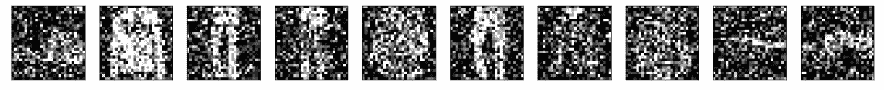 注意如何調整圖像的顯示形狀： ```py plt.figure(figsize=(20, 2)) for i in range(number_of_items): display = plt.subplot(1, number_of_items,i+1) plt.imshow(test_x_noisy[i].reshape(28, 28)) plt.gray() display.get_xaxis().set_visible(False) display.get_yaxis().set_visible(False) plt.show() ``` 這是結果，如以下屏幕快照所示：  因此很明顯，原始圖像與噪點幾乎沒有區別。 # 創建編碼層 接下來，我們創建編碼和解碼層。 我們將使用 Keras 函數式 API 風格來設置模型。 我們從一個占位符開始，以（下一個）卷積層所需的格式輸入： ```py input_image = Input(shape=(28, 28, 1)) ``` 接下來，我們有一個卷積層。 回憶卷積層的簽名： ```py Conv2D(filters, kernel_size, strides=(1, 1), padding='valid', data_format=None, dilation_rate=(1, 1), activation=None, use_bias=True, kernel_initializer='glorot_uniform', bias_initializer='zeros', kernel_regularizer=None, bias_regularizer=None, activity_regularizer=None, kernel_constraint=None, bias_constraint=None, **kwargs) ``` 我們將主要使用默認值； 接下來是我們的第一個`Conv2D`。 注意`(3,3)`的內核大小； 這是 Keras 應用于輸入圖像的滑動窗口的大小。 還記得`padding='same'`表示圖像用 0 左右填充，因此卷積的輸入和輸出層是內核（過濾器）以其中心“面板”開始于圖像中第一個像素時的大小。 。 默認步幅`(1, 1)`表示滑動窗口一次從圖像的左側到末尾水平移動一個像素，然后向下移動一個像素，依此類推。 接下來，我們將研究每個層的形狀，如下所示： ```py im = Conv2D(filters=32, kernel_size=(3, 3), activation='relu', padding='same')(input_image) print(x.shape) ``` 得到以下結果： ```py (?, 28, 28, 32) ``` `?`代表輸入項目的數量。 接下來，我們有一個`MaxPooling2D`層。 回想一下，在此情況下，此操作將在圖像上移動`(2, 2)`大小的滑動窗口，并采用在每個窗口中找到的最大值。 其簽名如下： ```py MaxPooling2D(pool_size=(2, 2), strides=None, padding='valid', data_format=None, **kwargs) ``` 這是下采樣的示例，因為生成的圖像尺寸減小了。 我們將使用以下代碼： ```py im = MaxPooling2D((2, 2), padding='same')(im) print(im.shape) ``` 得到以下結果： ```py (?, 14, 14, 32) ``` 其余的編碼層如下： ```py im = Conv2D(32, (3, 3), activation='relu', padding='same')(im) print(im.shape) encoded = MaxPooling2D((2, 2), padding='same')(im) print(encoded.shape) ``` 所有這些都結束了編碼。 # 創建解碼層 為了進行解碼，我們反轉了該過程，并使用上采樣層`UpSampling2D`代替了最大池化層。 上采樣層分別按大小[0]和大小[1]復制數據的行和列。 因此，在這種情況下，*會取消*最大合并層的效果，盡管會損失細粒度。 簽名如下： ```py UpSampling2D(size=(2, 2), data_format=None, **kwargs) ``` 我們使用以下內容： ```py im = UpSampling2D((2, 2))(im) ``` 以下是解碼層： ```py im = Conv2D(32, (3, 3), activation='relu', padding='same')(encoded) print(im.shape) im = UpSampling2D((2, 2))(im) print(im.shape) im = Conv2D(32, (3, 3), activation='relu', padding='same')(im) print(im.shape) im = UpSampling2D((2, 2))(im) print(im.shape) decoded = Conv2D(1, (3, 3), activation='sigmoid', padding='same')(im) print(decoded.shape) ``` 得到以下結果： ```py (?, 7, 7, 32) (?, 14, 14, 32) (?, 14, 14, 32) (?, 28, 28, 32) (?, 28, 28, 1) ``` 因此，您可以看到解碼層如何逆轉編碼層的過程。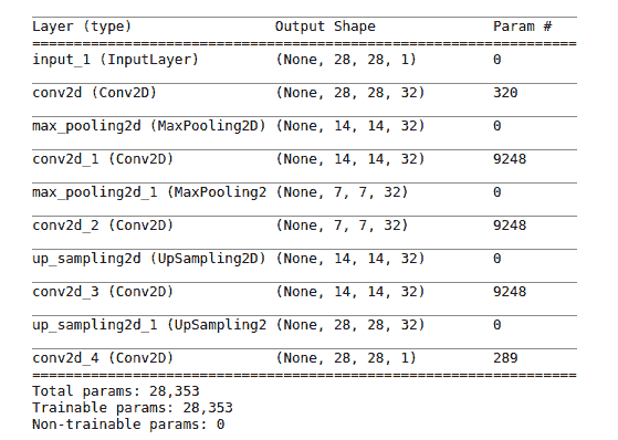 # 模型摘要 這是我們模型的摘要：  看看我們如何得出參數數字很有啟發性。 公式是參數數量 = 過濾器數量 x 內核大小 x 上一層的深度 + 過濾器數量（用于偏差）： * `input_1`：這是一個占位符，沒有可訓練的參數 * `conv2d`：過濾器數量`= 32`，內核大小`= 3 * 3 = 9`，上一層的深度`= 1`，因此`32 * 9 + 32 = 320` * `max_pooling2d`：最大池化層沒有可訓練的參數。 * `conv2d_1`：過濾器數`= 32`，內核大小`= 3 * 3 = 9`，上一層的深度`= 14`，因此`32 * 9 * 32 + 32 = 9,248` * `conv_2d_2`，`conv2d_3`：與`conv2d_1`相同 * `conv2d_4`：`1 * 9 * 32 + 1 = 289` # 模型實例化，編譯和訓練 接下來，我們用輸入層和輸出層實例化模型，然后使用`.compile`方法設置模型以進行訓練： ```py autoencoder = Model(inputs=input_img, outputs=decoded) autoencoder.compile(optimizer='adadelta', loss='binary_crossentropy') ``` 現在，我們準備訓練模型以嘗試恢復時尚商品的圖像。 請注意，我們已經為 TensorBoard 提供了回調，因此我們可以看一下一些訓練指標。 Keras TensorBoard 簽名如下： ```py keras.callbacks.TensorBoard( ["log_dir='./logs'", 'histogram_freq=0', 'batch_size=32', 'write_graph=True', 'write_grads=False', 'write_images=False', 'embeddings_freq=0', 'embeddings_layer_names=None', 'embeddings_metadata=None', 'embeddings_data=None', "update_freq='epoch'"], ) ``` 我們將主要使用默認值，如下所示： ```py tb = [TensorBoard(log_dir='./tmp/tb', write_graph=True)] ``` 接下來，我們使用`.fit()`方法訓練自編碼器。 以下代碼是其簽名： ```py fit(x=None, y=None, batch_size=None, epochs=1, verbose=1, callbacks=None, validation_split=0.0, validation_data=None, shuffle=True, class_weight=None, sample_weight=None, initial_epoch=0, steps_per_epoch=None, validation_steps=None, validation_freq=1) ``` 注意我們如何將`x_train_noisy`用于特征（輸入），并將`x_train`用于標簽（輸出）： ```py epochs=100 batch_size=128 autoencoder.fit(x_train_noisy, x_train, epochs=epochs,batch_size=batch_size, shuffle=True, validation_data=(x_test_noisy, x_test), callbacks=tb) ``` # 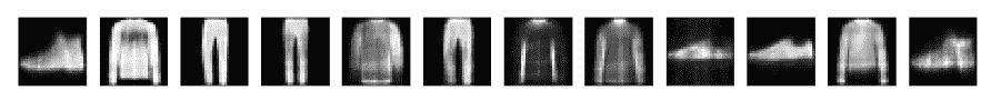去噪圖像 現在，通過解碼以下第一行中的所有測試集，然后循環遍歷一個固定數字（`number_of_items`）并顯示它們，來對測試集中的一些噪點圖像進行去噪。 請注意，在顯示每個圖像（`im`）之前，需要對其進行重塑： ```py decoded_images = autoencoder.predict(test_noisy_x) number_of_items = 10 plt.figure(figsize=(20, 2)) for item in range(number_of_items): display = plt.subplot(1, number_of_items,item+1) im = decoded_images[item].reshape(28, 28) plt.imshow(im, cmap="gray") display.get_xaxis().set_visible(False) display.get_yaxis().set_visible(False) plt.show() ``` 我們得到以下結果：  考慮到圖像最初模糊的程度，降噪器已經做了合理的嘗試來恢復圖像。 # TensorBoard 輸出 要查看 TensorBoard 輸出，請在命令行上使用以下命令： ```py tensorboard --logdir=./tmp/tb ``` 然后，您需要將瀏覽器指向`http://localhost:6006`。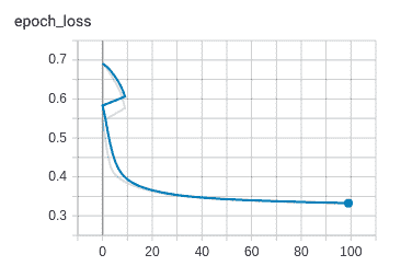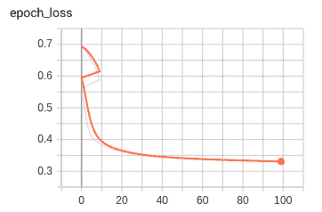 下圖顯示了作為訓練和驗證時間的函數（`x`軸）的損失（`y`軸）： 下圖顯示了訓練損失：  驗證損失如下圖所示：  到此結束我們對自編碼器的研究。 # 總結 在本章中，我們研究了自編碼器在無監督學習中的兩種應用：首先用于壓縮數據，其次用于降噪，這意味著從圖像中去除噪聲。 在下一章中，我們將研究如何在圖像處理和識別中使用神經網絡。