八、TensorFlow 和 Keras 中的用于文本數據的 RNN · ApacheCN 深度學習譯文集

# 八、TensorFlow 和 Keras 中的用于文本數據的 RNN 文本數據可以被視為一系列字符，單詞，句子或段落。 **循環神經網絡**（**RNN**）已被證明是非常有用的序列神經網絡結構。為了將神經網絡模型應用于**自然語言處理**（**NLP**）任務，文本被視為單詞序列。事實證明，這對于 NLP 任務非常成功，例如： * 問題回答 * 會話智能體或聊天機器人 * 文本分類 * 情感分析 * 圖像標題或描述文本生成 * 命名實體識別 * 語音識別和標記 NLP 與 TensorFlow 深度學習技術是一個廣闊的領域，很難在一章中捕捉到。因此，我們嘗試使用 Tensorflow 和 Keras 為您提供該領域中最流行和最重要的示例。一旦掌握了本章的內容，不要忘記探索和試驗 NLP 的其他領域。在本章中，我們將了解以下主題： * 詞向量表示 * 為 word2vec 模型準備數據 * TensorFlow 和 Keras 中的 SkipGram 模型 * 使用 t-SNE 可視化單詞嵌入 * TensorFlow 和 Keras 中使用 LSTM 模型的文本生成示例 # 詞向量表示為了從文本數據中學習神經網絡模型的參數，首先，我們必須將文本或自然語言數據轉換為可由神經網絡攝取的格式。神經網絡通常以數字向量的形式攝取文本。將原始文本數據轉換為數字向量的算法稱為字嵌入算法。一種流行的字嵌入方法是我們在 MNIST 圖像分類中看到的**單熱編碼**。假設我們的文本數據集由 60,000 個字典單詞組成。然后，每個單詞可以由具有 60,000 個元素的單熱編碼向量表示，其中除了表示具有值 1 的該單詞的一個元素之外，所有其他元素具有零值。然而，單熱編碼方法有其缺點。首先，對于具有大量單詞的詞匯，單熱詞向量的維數變得非常大。其次，人們無法找到與單熱編碼向量的單詞相似性。例如，假設貓和小貓的向量分別為`[1 0 0 0 0 0]`和`[0 0 0 0 0 1]`。這些向量沒有相似之處。還有其他基于語料庫的方法，用于將基于文本的語料庫轉換為數字向量，例如： * 單詞頻率 - 反向文檔頻率（TF-IDF） * 潛在語義分析（LSA） * 主題建模最近，用數值向量表示單詞的焦點已轉移到基于分布假設的方法，這意味著具有相似語義含義的單詞傾向于出現在類似的上下文中。兩種最廣泛使用的方法稱為 word2vec 和 GloVe。我們將在本章中使用 word2vec 進行練習。正如我們在前一段中所了解到的，單熱編碼給出了語料庫字典中單詞總數大小的維數。使用 word2vec 創建的單詞向量的維度要低得多。 word2vec 系列模型使用兩種架構構建： * **CBOW**：訓練模型以學習給定上下文詞的中心詞的概率分布。因此，給定一組上下文單詞，模型以您在高中語言課程中所做的填空方式預測中心單詞。 CBOW 架構最適用于具有較小詞匯表的數據集。 * **SkipGram**：訓練模型以學習給定中心詞的上下文詞的概率分布。因此，給定一個中心詞，模型以您在高中語言課程中完成的句子方式預測語境詞。例如，讓我們考慮一下這句話： ``` Vets2data.org is a non-profit for educating the US Military Veterans Community on Artificial Intelligence and Data Science. ``` 在 CBOW 架構中，給出單詞`Military`和`Community`，模型學習單詞`Veterans`的概率，并在 SkipGram 架構中，給出單詞`Veterans`，模型學習單詞`Military`和`Community`的概率。 word2vec 模型以無監督的方式從文本語料庫中學習單詞向量。文本語料庫分為成對的上下文單詞和目標單詞。雖然這些對是真正的對，但是偽對是用隨機配對的上下文詞和上下文詞生成的，因此在數據中產生噪聲。訓練分類器以學習用于區分真對和假對的參數。該分類器的參數成為 word2vec 模型或單詞向量。關于 word2vec 理論背后的數學和理論的更多信息可以從以下論文中學到： ``` Mikolov, T., I. Sutskever, K. Chen, G. Corrado, and J. Dean. Distributed Representations of Words and Phrases and Their Compositionality.?_Advances in Neural Information Processing Systems_, 2013, pp. 3111–3119. Mikolov, T., K. Chen, G. Corrado, and J. Dean. Efficient Estimation of Word Representations in Vector Space.?_arXiv_, 2013, pp. 1–12. Rong, X. word2vec Parameter Learning Explained.?_arXiv:1411.2738_, 2014, pp. 1–19. Baroni, M., G. Dinu, and G. Kruszewski. Don’t Count, Predict! A Systematic Comparison of Context-Counting vs. Context-Predicting Semantic Vectors. 2014. ``` 您應該使用 GloVe 和 word2vec 練習并應用適用于您的文本數據的方法。有關 GLoVe 算法的更多信息可以從以下文章中學習： ``` Pennington, J., R. Socher, and C. Manning. GloVe: Global Vectors for Word Representation. 2014. ``` 讓我們通過在 TensorFlow 和 Keras 中創建單詞向量來理解 word2vec 模型。您可以按照 Jupyter 筆記本中的下幾節的代碼`ch-08a_Embeddings_in_TensorFlow_and_Keras`。 # 用于 word2vec 模型的數據準備我們將使用流行的 PTB 和 text8 數據集進行演示。 **PennTreebank**（**PTB**）數據集是在 UPenn 進行的 [Penn Treebank 項目](https://catalog.ldc.upenn.edu/ldc99t42)的副產品。 PTB 項目團隊在華爾街日報三年的故事中提取了大約一百萬字，并以 Treebank II 風格對其進行了標注。 PTB 數據集有兩種形式：基本示例，大小約為 35 MB，高級示例，大小約為 235 MB。我們將使用由 929K 字組成的簡單數據集進行訓練，73K 字用于驗證，82K 字用于測試。建議您瀏覽高級數據集。有關 PTB 數據集的更多詳細信息，[請訪問此鏈接](http://www.fit.vutbr.cz/~imikolov/rnnlm/simple-examples.tgz) 。 [可以從此鏈接下載 PTB 數據集](http://www.fit.vutbr.cz/~imikolov/rnnlm/rnn-rt07-example.tar.gz)。 **text8** 數據集是一個較短的清理版本的大型維基百科數據轉儲，大小約為 1GB。有關如何創建 text8 數據集的過程，[請參見此鏈接](http://mattmahoney.net/dc/textdata.html)。 [text8 數據集可以從此鏈接下載](http://mattmahoney.net/dc/text8.zip)。使用我們的自定義庫`datasetslib`中的`load_data`代碼加載數據集： `load_data()`函數執行以下操作： 1. 如果數據集的 URL 在本地不可用，它將從數據集的 URL 下載數據存檔。 2. 由于`PTB`數據有三個文件，它首先從訓練文件中讀取文本，而對于`text8`，它從歸檔中讀取第一個文件。 3. 它將訓練文件中的單詞轉換為詞匯表，并為每個詞匯單詞分配一個唯一的數字，單詞 ID，將其存儲在集合`word2id`中，并準備反向詞典，這樣我們就可以從 ID 中查找單詞，并將其存儲在集合`id2word`中。 1. 它使用集合`word2id`將文本文件轉換為 ID 序列。 2. 因此，在`load_data`的末尾，我們在訓練數據集中有一系列數字，在集合`id2word`中有一個 ID 到字的映射。讓我們看一下從 text8 和 PTB 數據集加載的數據： # 加載和準備 PTB 數據集首先導入模塊并加載數據如下:: ```py from datasetslib.ptb import PTBSimple ptb = PTBSimple() # downloads data, converts words to ids, converts files to a list of ids ptb.load_data() print('Train :',ptb.part['train'][0:5]) print('Test: ',ptb.part['test'][0:5]) print('Valid: ',ptb.part['valid'][0:5]) print('Vocabulary Length = ',ptb.vocab_len) ``` 每個數據集的前五個元素以及詞匯長度打印如下： ```py Train : [9970, 9971, 9972, 9974, 9975] Test: [102, 14, 24, 32, 752] Valid: [1132, 93, 358, 5, 329] Vocabulary Length = 10000 ``` 我們將上下文窗口設置為兩個單詞并獲得 CBOW 對： ```py ptb.skip_window=2 ptb.reset_index_in_epoch() # in CBOW input is the context word and output is the target word y_batch, x_batch = ptb.next_batch_cbow() print('The CBOW pairs : context,target') for i in range(5 * ptb.skip_window): print('(', [ptb.id2word[x_i] for x_i in x_batch[i]], ',', y_batch[i], ptb.id2word[y_batch[i]], ')') ``` 輸出是： ```py The CBOW pairs : context,target ( ['aer', 'banknote', 'calloway', 'centrust'] , 9972 berlitz ) ( ['banknote', 'berlitz', 'centrust', 'cluett'] , 9974 calloway ) ( ['berlitz', 'calloway', 'cluett', 'fromstein'] , 9975 centrust ) ( ['calloway', 'centrust', 'fromstein', 'gitano'] , 9976 cluett ) ( ['centrust', 'cluett', 'gitano', 'guterman'] , 9980 fromstein ) ( ['cluett', 'fromstein', 'guterman', 'hydro-quebec'] , 9981 gitano ) ( ['fromstein', 'gitano', 'hydro-quebec', 'ipo'] , 9982 guterman ) ( ['gitano', 'guterman', 'ipo', 'kia'] , 9983 hydro-quebec ) ( ['guterman', 'hydro-quebec', 'kia', 'memotec'] , 9984 ipo ) ( ['hydro-quebec', 'ipo', 'memotec', 'mlx'] , 9986 kia ) ``` 現在讓我們看看 SkipGram 對： ```py ptb.skip_window=2 ptb.reset_index_in_epoch() # in SkipGram input is the target word and output is the context word x_batch, y_batch = ptb.next_batch() print('The SkipGram pairs : target,context') for i in range(5 * ptb.skip_window): print('(',x_batch[i], ptb.id2word[x_batch[i]], ',', y_batch[i], ptb.id2word[y_batch[i]],')') ``` 輸出為： ```py The SkipGram pairs : target,context ( 9972 berlitz , 9970 aer ) ( 9972 berlitz , 9971 banknote ) ( 9972 berlitz , 9974 calloway ) ( 9972 berlitz , 9975 centrust ) ( 9974 calloway , 9971 banknote ) ( 9974 calloway , 9972 berlitz ) ( 9974 calloway , 9975 centrust ) ( 9974 calloway , 9976 cluett ) ( 9975 centrust , 9972 berlitz ) ( 9975 centrust , 9974 calloway ) ``` # 加載和準備 text8 數據集現在我們使用 text8 數據集執行相同的加載和預處理步驟： ```py from datasetslib.text8 import Text8 text8 = Text8() text8.load_data() # downloads data, converts words to ids, converts files to a list of ids print('Train:', text8.part['train'][0:5]) print('Vocabulary Length = ',text8.vocab_len) ``` 我們發現詞匯長度大約是 254,000 字： ```py Train: [5233, 3083, 11, 5, 194] Vocabulary Length = 253854 ``` 一些教程通過查找最常用的單詞或將詞匯量大小截斷為 10,000 個單詞來操縱此數據。但是，我們使用了 text8 數據集的第一個文件中的完整數據集和完整詞匯表。準備 CBOW 對： ```py text8.skip_window=2 text8.reset_index_in_epoch() # in CBOW input is the context word and output is the target word y_batch, x_batch = text8.next_batch_cbow() print('The CBOW pairs : context,target') for i in range(5 * text8.skip_window): print('(', [text8.id2word[x_i] for x_i in x_batch[i]], ',', y_batch[i], text8.id2word[y_batch[i]], ')') ``` 輸出是： ```py The CBOW pairs : context,target ( ['anarchism', 'originated', 'a', 'term'] , 11 as ) ( ['originated', 'as', 'term', 'of'] , 5 a ) ( ['as', 'a', 'of', 'abuse'] , 194 term ) ( ['a', 'term', 'abuse', 'first'] , 1 of ) ( ['term', 'of', 'first', 'used'] , 3133 abuse ) ( ['of', 'abuse', 'used', 'against'] , 45 first ) ( ['abuse', 'first', 'against', 'early'] , 58 used ) ( ['first', 'used', 'early', 'working'] , 155 against ) ( ['used', 'against', 'working', 'class'] , 127 early ) ( ['against', 'early', 'class', 'radicals'] , 741 working ) ``` 準備 SkipGram 對： ```py text8.skip_window=2 text8.reset_index_in_epoch() # in SkipGram input is the target word and output is the context word x_batch, y_batch = text8.next_batch() print('The SkipGram pairs : target,context') for i in range(5 * text8.skip_window): print('(',x_batch[i], text8.id2word[x_batch[i]], ',', y_batch[i], text8.id2word[y_batch[i]],')') ``` 輸出為： ```py The SkipGram pairs : target,context ( 11 as , 5233 anarchism ) ( 11 as , 3083 originated ) ( 11 as , 5 a ) ( 11 as , 194 term ) ( 5 a , 3083 originated ) ( 5 a , 11 as ) ( 5 a , 194 term ) ( 5 a , 1 of ) ( 194 term , 11 as ) ( 194 term , 5 a ) ``` # 準備小驗證集為了演示該示例，我們創建了一個包含 8 個單詞的小型驗證集，每個單詞是從單詞中隨機選擇的，其中單詞 ID 在 0 到`10 x 8`之間。 ```py valid_size = 8 x_valid = np.random.choice(valid_size * 10, valid_size, replace=False) print(x_valid) ``` 作為示例，我們將以下內容作為驗證集： ```py valid: [64 58 59 4 69 53 31 77] ``` 我們將使用此驗證集通過打印五個最接近的單詞來演示嵌入一詞的結果。 # TensorFlow 中的 SkipGram 模型現在我們已經準備好了訓練和驗證數據，讓我們在 TensorFlow 中創建一個 SkipGram 模型。我們首先定義超參數： ```py batch_size = 128 embedding_size = 128 skip_window = 2 n_negative_samples = 64 ptb.skip_window=2 learning_rate = 1.0 ``` * `batch_size`是要在單個批次中輸入算法的目標和上下文單詞對的數量 * `embedding_size`是每個單詞的單詞向量或嵌入的維度 * `ptb.skip_window`是在兩個方向上的目標詞的上下文中要考慮的詞的數量 * `n_negative_samples`是由 NCE 損失函數生成的負樣本數，本章將進一步說明在一些教程中，包括 TensorFlow 文檔中的一個教程，還使用了一個參數`num_skips`。在這樣的教程中，作者選擇了`num_skips`（目標，上下文）對。例如，如果`skip_window`是 2，那么對的總數將是 4，如果`num_skips`被設置為 2，則只有兩對將被隨機選擇用于訓練。但是，我們考慮了所有的對以便保持訓練練習簡單。定義訓練數據的輸入和輸出占位符以及驗證數據的張量： ```py inputs = tf.placeholder(dtype=tf.int32, shape=[batch_size]) outputs = tf.placeholder(dtype=tf.int32, shape=[batch_size,1]) inputs_valid = tf.constant(x_valid, dtype=tf.int32) ``` 定義一個嵌入矩陣，其行數等于詞匯長度，列等于嵌入維度。該矩陣中的每一行將表示詞匯表中一個單詞的單詞向量。使用在 -1.0 到 1.0 之間均勻采樣的值填充此嵌入矩陣。 ```py # define embeddings matrix with vocab_len rows and embedding_size columns # each row represents vectore representation or embedding of a word # in the vocbulary embed_dist = tf.random_uniform(shape=[ptb.vocab_len, embedding_size], minval=-1.0,maxval=1.0) embed_matrix = tf.Variable(embed_dist,name='embed_matrix') ``` 使用此矩陣，定義使用`tf.nn.embedding_lookup()`實現的嵌入查找表。`tf.nn.embedding_lookup()`有兩個參數：嵌入矩陣和輸入占位符。查找函數返回`inputs`占位符中單詞的單詞向量。 ```py # define the embedding lookup table # provides the embeddings of the word ids in the input tensor embed_ltable = tf.nn.embedding_lookup(embed_matrix, inputs) ``` `embed_ltable`也可以解釋為輸入層頂部的嵌入層。接下來，將嵌入層的輸出饋送到 softmax 或噪聲對比估計（NCE）層。 NCE 基于一個非常簡單的想法，即訓練基于邏輯回歸的二分類器，以便從真實和嘈雜數據的混合中學習參數。 [TensorFlow 文檔進一步詳細描述了 NCE](https://www.tensorflow.org/tutorials/word2vec#scaling_up_with_noise-contrastive_training)。總之，基于 softmax 損失的模型在計算上是昂貴的，因為在整個詞匯表中計算概率分布并對其進行歸一化。基于 NCE 損耗的模型將其減少為二分類問題，即從噪聲樣本中識別真實樣本。 NCE 的基本數學細節可以在以下 NIPS 論文中找到：使用噪聲對比估計高效學習詞嵌入，作者 Andriy Mnih 和 Koray Kavukcuoglu。[該論文可從此鏈接獲得](http://papers.nips.cc/paper/5165-learning-word-embeddings-efficiently-with-noise-contrastive-estimation.pdf)。 `tf.nn.nce_loss()`函數在求值計算損耗時自動生成負樣本：參數`num_sampled`設置為等于負樣本數（`n_negative_samples`）。此參數指定要繪制的負樣本數。 ```py # define noise-contrastive estimation (NCE) loss layer nce_dist = tf.truncated_normal(shape=[ptb.vocab_len, embedding_size], stddev=1.0 / tf.sqrt(embedding_size * 1.0) ) nce_w = tf.Variable(nce_dist) nce_b = tf.Variable(tf.zeros(shape=[ptb.vocab_len])) loss = tf.reduce_mean(tf.nn.nce_loss(weights=nce_w, biases=nce_b, inputs=embed_ltable, labels=outputs, num_sampled=n_negative_samples, num_classes=ptb.vocab_len ) ) ``` 接下來，計算驗證集中的樣本與嵌入矩陣之間的余弦相似度： 1. 為了計算相似性得分，首先，計算嵌入矩陣中每個單詞向量的 L2 范數。 ```py # Compute the cosine similarity between validation set samples # and all embeddings. norm = tf.sqrt(tf.reduce_sum(tf.square(embed_matrix), 1, keep_dims=True)) normalized_embeddings = embed_matrix / norm ``` 1. 查找驗證集中的樣本的嵌入或單詞向量： ```py embed_valid = tf.nn.embedding_lookup(normalized_embeddings, inputs_valid) ``` 1. 通過將驗證集的嵌入與嵌入矩陣相乘來計算相似性得分。 ```py similarity = tf.matmul( embed_valid, normalized_embeddings, transpose_b=True) ``` 這給出了具有（`valid_size`，`vocab_len`）形狀的張量。張量中的每一行指的是驗證詞和詞匯單詞之間的相似性得分。接下來，定義 SGD 優化器，學習率為 0.9，歷時 50 個周期。 ```py n_epochs = 10 learning_rate = 0.9 n_batches = ptb.n_batches(batch_size) optimizer = tf.train.GradientDescentOptimizer(learning_rate) .minimize(loss) ``` 對于每個周期： 1. 逐批在整個數據集上運行優化器。 ```py ptb.reset_index_in_epoch() for step in range(n_batches): x_batch, y_batch = ptb.next_batch() y_batch = dsu.to2d(y_batch,unit_axis=1) feed_dict = {inputs: x_batch, outputs: y_batch} _, batch_loss = tfs.run([optimizer, loss], feed_dict=feed_dict) epoch_loss += batch_loss ``` 1. 計算并打印周期的平均損失。 ```py epoch_loss = epoch_loss / n_batches print('\n','Average loss after epoch ', epoch, ': ', epoch_loss) ``` 1. 在周期結束時，計算相似性得分。 ```py similarity_scores = tfs.run(similarity) ``` 1. 對于驗證集中的每個單詞，打印具有最高相似性得分的五個單詞。 ```py top_k = 5 for i in range(valid_size): similar_words = (-similarity_scores[i,:]) .argsort()[1:top_k + 1] similar_str = 'Similar to {0:}:' .format(ptb.id2word[x_valid[i]]) for k in range(top_k): similar_str = '{0:} {1:},'.format(similar_str, ptb.id2word[similar_words[k]]) print(similar_str) ``` 最后，在完成所有周期之后，計算可在學習過程中進一步利用的嵌入向量： ```py final_embeddings = tfs.run(normalized_embeddings) ``` 完整的訓練代碼如下： ```py n_epochs = 10 learning_rate = 0.9 n_batches = ptb.n_batches_wv() optimizer = tf.train.GradientDescentOptimizer(learning_rate).minimize(loss) with tf.Session() as tfs: tf.global_variables_initializer().run() for epoch in range(n_epochs): epoch_loss = 0 ptb.reset_index() for step in range(n_batches): x_batch, y_batch = ptb.next_batch_sg() y_batch = nputil.to2d(y_batch, unit_axis=1) feed_dict = {inputs: x_batch, outputs: y_batch} _, batch_loss = tfs.run([optimizer, loss], feed_dict=feed_dict) epoch_loss += batch_loss epoch_loss = epoch_loss / n_batches print('\nAverage loss after epoch ', epoch, ': ', epoch_loss) # print closest words to validation set at end of every epoch similarity_scores = tfs.run(similarity) top_k = 5 for i in range(valid_size): similar_words = (-similarity_scores[i, :] ).argsort()[1:top_k + 1] similar_str = 'Similar to {0:}:'.format( ptb.id2word[x_valid[i]]) for k in range(top_k): similar_str = '{0:} {1:},'.format( similar_str, ptb.id2word[similar_words[k]]) print(similar_str) final_embeddings = tfs.run(normalized_embeddings) ``` 這是我們分別在第 1 和第 10 周期之后得到的輸出： ```py Average loss after epoch 0 : 115.644006802 Similar to we: types, downturn, internal, by, introduce, Similar to been: said, funds, mcgraw-hill, street, have, Similar to also: will, she, next, computer, 's, Similar to of: was, and, milk, dollars, $, Similar to last: be, october, acknowledging, requested, computer, Similar to u.s.: plant, increase, many, down, recent, Similar to an: commerce, you, some, american, a, Similar to trading: increased, describes, state, companies, in, Average loss after epoch 9 : 5.56538496033 Similar to we: types, downturn, introduce, internal, claims, Similar to been: exxon, said, problem, mcgraw-hill, street, Similar to also: will, she, ssangyong, audit, screens, Similar to of: seasonal, dollars, motor, none, deaths, Similar to last: acknowledging, allow, incorporated, joint, requested, Similar to u.s.: undersecretary, typically, maxwell, recent, increase, Similar to an: banking, officials, imbalances, americans, manager, Similar to trading: describes, increased, owners, committee, else, ``` 最后，我們運行 5000 個周期的模型并獲得以下結果： ```py Average loss after epoch 4999 : 2.74216903135 Similar to we: matter, noted, here, classified, orders, Similar to been: good, precedent, medium-sized, gradual, useful, Similar to also: introduce, england, index, able, then, Similar to of: indicator, cleveland, theory, the, load, Similar to last: dec., office, chrysler, march, receiving, Similar to u.s.: label, fannie, pressures, squeezed, reflection, Similar to an: knowing, outlawed, milestones, doubled, base, Similar to trading: associates, downturn, money, portfolios, go, ``` 嘗試進一步運行，最多 50,000 個周期，以獲得更好的結果。同樣，我們在 50 個周期之后使用 text8 模型得到以下結果： ```py Average loss after epoch 49 : 5.74381046423 Similar to four: five, three, six, seven, eight, Similar to all: many, both, some, various, these, Similar to between: with, through, thus, among, within, Similar to a: another, the, any, each, tpvgames, Similar to that: which, however, although, but, when, Similar to zero: five, three, six, eight, four, Similar to is: was, are, has, being, busan, Similar to no: any, only, the, another, trinomial, ``` # t-SNE 和單詞嵌入可視化讓我們可視化我們在上一節中生成的單詞嵌入。 t-SNE 是在二維空間中顯示高維數據的最流行的方法。我們將使用 scikit-learn 庫中的方法，并重用 TensorFlow 文檔中給出的代碼，來繪制我們剛學過的詞嵌入的圖形。 [TensorFlow 文檔中的原始代碼可從此鏈接獲得](https://github.com/tensorflow/tensorflow/blob/r1.3/tensorflow/examples/tutorials/word2vec/word2vec_basic.py)。以下是我們如何實現該程序： 1. 創建`tsne`模型： ```py tsne = TSNE(perplexity=30, n_components=2, init='pca', n_iter=5000, method='exact') ``` 1. 將要顯示的嵌入數限制為 500，否則，圖形變得非常難以理解： ```py n_embeddings = 500 ``` 1. 通過調用`tsne`模型上的`fit_transform()`方法并將`final_embeddings`的第一個`n_embeddings`作為輸入來創建低維表示。 ```py low_dim_embeddings = tsne.fit_transform( final_embeddings[:n_embeddings, :]) ``` 1. 找到我們為圖表選擇的單詞向量的文本表示： ```py labels = [ptb.id2word[i] for i in range(n_embeddings)] ``` 1. 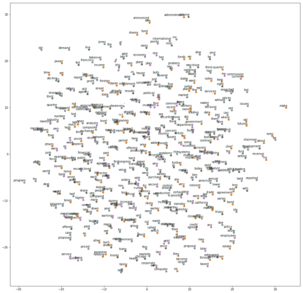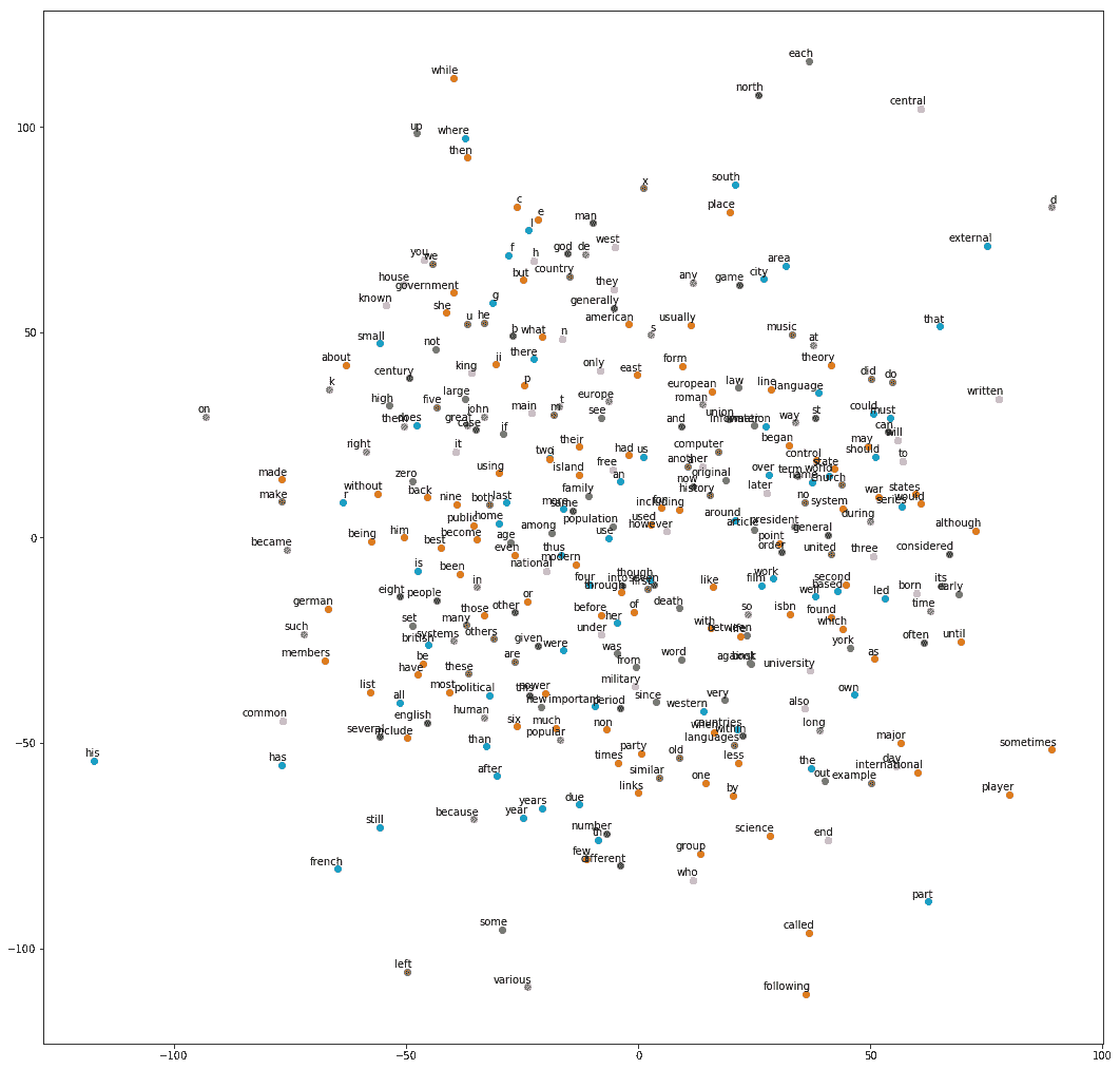最后，繪制嵌入圖： ```py plot_with_labels(low_dim_embeddings, labels) ``` 我們得到以下繪圖： ![](https://img.kancloud.cn/39/00/3900e73576bc929ef85e83594244985b_1050x1013.png)t-SNE visualization of embeddings for PTB data set 同樣，從 text8 模型中，我們得到以下圖： ![](https://img.kancloud.cn/e9/d6/e9d6ce5f402bc112cd513f93e871822b_1062x1013.png)t-SNE visualization of embeddings for text8 data set # Keras 中的 SkipGram 模型使用 Keras 的嵌入模型的流程與 TensorFlow 保持一致。 * 在 Keras 函數式或順序模型中創建網絡架構 * 將目標和上下文單詞的真實性對提供給網絡 * 查找目標和上下文單詞的單詞向量 * 執行單詞向量的點積來獲得相似性得分 * 將相似性得分通過 sigmoid 層以將輸出作為真或假對現在讓我們使用 Keras 函數式 API 實現這些步驟： 1. 導入所需的庫： ```py from keras.models import Model from keras.layers.embeddings import Embedding from keras.preprocessing import sequence from keras.preprocessing.sequence import skipgrams from keras.layers import Input, Dense, Reshape, Dot, merge import keras ``` 重置圖，以便清除以前在 Jupyter 筆記本中運行的任何后續效果： ```py # reset the jupyter buffers tf.reset_default_graph() keras.backend.clear_session() ``` 1. 創建一個驗證集，我們將用它來打印我們的模型在訓練結束時找到的相似單詞： ```py valid_size = 8 x_valid = np.random.choice(valid_size * 10, valid_size, replace=False) print('valid: ',x_valid) ``` 1. 定義所需的超參數： ```py batch_size = 1024 embedding_size = 512 n_negative_samples = 64 ptb.skip_window=2 ``` 1. 使用`keras.preprocessing.sequence`中的`make_sampling_table()`函數創建一個大小等于詞匯長度的樣本表。接下來，使用`keras.preprocessing.sequence`中的函數`skipgrams()`生成上下文和目標詞對以及表示它們是真對還是假對的標簽。 ```py sample_table = sequence.make_sampling_table(ptb.vocab_len) pairs, labels= sequence.skipgrams(ptb.part['train'], ptb.vocab_len,window_size=ptb.skip_window, sampling_table=sample_table) ``` 1. 讓我們打印一些使用以下代碼生成的偽造和真實對： ```py print('The SkipGram pairs : target,context') for i in range(5 * ptb.skip_window): print(['{} {}'.format(id,ptb.id2word[id]) \ for id in pairs[i]],':',labels[i]) ``` 對配對如下： ```py The SkipGram pairs : target,context ['547 trying', '5 to'] : 1 ['4845 bargain', '2 <eos>'] : 1 ['1705 election', '198 during'] : 1 ['4704 flows', '8117 gun'] : 0 ['13 is', '37 company'] : 1 ['625 above', '132 three'] : 1 ['5768 pessimistic', '1934 immediate'] : 0 ['637 china', '2 <eos>'] : 1 ['258 five', '1345 pence'] : 1 ['1956 chrysler', '8928 exercises'] : 0 ``` 1. 從上面生成的對中拆分目標和上下文單詞，以便將它們輸入模型。將目標和上下文單詞轉換為二維數組。 ```py x,y=zip(*pairs) x=np.array(x,dtype=np.int32) x=dsu.to2d(x,unit_axis=1) y=np.array(y,dtype=np.int32) y=dsu.to2d(y,unit_axis=1) labels=np.array(labels,dtype=np.int32) labels=dsu.to2d(labels,unit_axis=1) ``` 1. 定義網絡的架構。正如我們所討論的，必須將目標和上下文單詞輸入網絡，并且需要從嵌入層中查找它們的向量。因此，首先我們分別為目標和上下文單詞定義輸入，嵌入和重塑層： ```py # build the target word model target_in = Input(shape=(1,),name='target_in') target = Embedding(ptb.vocab_len,embedding_size,input_length=1, name='target_em')(target_in) target = Reshape((embedding_size,1),name='target_re')(target) # build the context word model context_in = Input((1,),name='context_in') context = Embedding(ptb.vocab_len,embedding_size,input_length=1, name='context_em')(context_in) context = Reshape((embedding_size,1),name='context_re')(context) ``` 1. 接下來，構建這兩個模型的點積，將其輸入 sigmoid 層以生成輸出標簽： ```py # merge the models with the dot product to check for # similarity and add sigmoid layer output = Dot(axes=1,name='output_dot')([target,context]) output = Reshape((1,),name='output_re')(output) output = Dense(1, activation='sigmoid',name='output_sig')(output) ``` 1. 從我們剛剛創建的輸入和輸出模型構建函數式模型： ```py # create the functional model for finding word vectors model = Model(inputs=[target_in,context_in],outputs=output) model.compile(loss='binary_crossentropy', optimizer='adam') ``` 1. 此外，在給定輸入目標詞的情況下，構建一個模型，用于預測與所有單詞的相似性： ```py # merge the models and create model to check for cosine similarity similarity = Dot(axes=0,normalize=True, name='sim_dot')([target,context]) similarity_model = Model(inputs=[target_in,context_in], outputs=similarity) ``` 讓我們打印模型摘要： ```py __________________________________________________________________________ Layer (type) Output Shape Param # Connected to ========================================================================== target_in (InputLayer) (None, 1) 0 __________________________________________________________________________ context_in (InputLayer) (None, 1) 0 __________________________________________________________________________ target_em (Embedding) (None, 1, 512) 5120000 target_in[0][0] __________________________________________________________________________ context_em (Embedding) (None, 1, 512) 5120000 context_in[0][0] __________________________________________________________________________ target_re (Reshape) (None, 512, 1) 0 target_em[0][0] __________________________________________________________________________ context_re (Reshape) (None, 512, 1) 0 context_em[0][0] __________________________________________________________________________ output_dot (Dot) (None, 1, 1) 0 target_re[0][0] context_re[0][0] __________________________________________________________________________ output_re (Reshape) (None, 1) 0 output_dot[0][0] __________________________________________________________________________ output_sig (Dense) (None, 1) 2 output_re[0][0] ========================================================================== Total params: 10,240,002 Trainable params: 10,240,002 Non-trainable params: 0 __________________________________________________________________________ ``` 1. 接下來，訓練模型。我們只訓練了 5 個周期，但你應該嘗試更多的周期，至少 1000 或 10,000 個周期。請記住，這將需要幾個小時，因為這不是最優化的代碼。歡迎您使用本書和其他來源的提示和技巧進一步優化代碼。 ```py n_epochs = 5 batch_size = 1024 model.fit([x,y],labels,batch_size=batch_size, epochs=n_epochs) ``` 讓我們根據這個模型發現的單詞向量打印單詞的相似度： ```py # print closest words to validation set at end of training top_k = 5 y_val = np.arange(ptb.vocab_len, dtype=np.int32) y_val = dsu.to2d(y_val,unit_axis=1) for i in range(valid_size): x_val = np.full(shape=(ptb.vocab_len,1),fill_value=x_valid[i], dtype=np.int32) similarity_scores = similarity_model.predict([x_val,y_val]) similarity_scores=similarity_scores.flatten() similar_words = (-similarity_scores).argsort()[1:top_k + 1] similar_str = 'Similar to {0:}:'.format(ptb.id2word[x_valid[i]]) for k in range(top_k): similar_str = '{0:} {1:},'.format(similar_str, ptb.id2word[similar_words[k]]) print(similar_str) ``` 我們得到以下輸出： ```py Similar to we: rake, kia, sim, ssangyong, memotec, Similar to been: nahb, sim, rake, punts, rubens, Similar to also: photography, snack-food, rubens, nahb, ssangyong, Similar to of: isi, rake, memotec, kia, mlx, Similar to last: rubens, punts, memotec, sim, photography, Similar to u.s.: mlx, memotec, punts, rubens, kia, Similar to an: memotec, isi, ssangyong, rake, sim, Similar to trading: rake, rubens, swapo, mlx, nahb, ``` 到目前為止，我們已經看到了如何使用 TensorFlow 及其高級庫 Keras 創建單詞向量或嵌入。現在讓我們看看如何使用 TensorFlow 和 Keras 來學習模型并將模型應用于一些與 NLP 相關的任務的預測。 # TensorFlow 和 Keras 中的 RNN 模型和文本生成文本生成是 NLP 中 RNN 模型的主要應用之一。針對文本序列訓練 RNN 模型，然后通過提供種子文本作為輸入來生成文本序列。讓我們試試 text8 數據集。讓我們加載 text8 數據集并打印前 100 個單詞： ```py from datasetslib.text8 import Text8 text8 = Text8() # downloads data, converts words to ids, converts files to a list of ids text8.load_data() print(' '.join([text8.id2word[x_i] for x_i in text8.part['train'][0:100]])) ``` 我們得到以下輸出： ```py anarchism originated as a term of abuse first used against early working class radicals including the diggers of the english revolution and the sans culottes of the french revolution whilst the term is still used in a pejorative way to describe any act that used violent means to destroy the organization of society it has also been taken up as a positive label by self defined anarchists the word anarchism is derived from the greek without archons ruler chief king anarchism as a political philosophy is the belief that rulers are unnecessary and should be abolished although there are differing ``` 在我們的筆記本示例中，我們將數據加載剪切為 5,000 字的文本，因為較大的文本需要高級技術，例如分布式或批量，我們希望保持示例簡單。 ```py from datasetslib.text8 import Text8 text8 = Text8() text8.load_data(clip_at=5000) print('Train:', text8.part['train'][0:5]) print('Vocabulary Length = ',text8.vocab_len) ``` 我們看到詞匯量現在減少到 1,457 個單詞。 ```py Train: [ 8 497 7 5 116] Vocabulary Length = 1457 ``` 在我們的示例中，我們構造了一個非常簡單的單層 LSTM。為了訓練模型，我們使用 5 個單詞作為輸入來學習第六個單詞的參數。輸入層是 5 個字，隱藏層是具有 128 個單元的 LSTM 單元，最后一層是完全連接的層，其輸出等于詞匯量大小。由于我們正在演示這個例子，我們沒有使用單詞向量，而是使用非常簡單的單熱編碼輸出向量。一旦模型被訓練，我們用 2 個不同的字符串作為生成更多字符的種子來測試它： * `random5`：隨機選擇 5 個單詞生成的字符串。 * `first5`：從文本的前 5 個單詞生成的字符串。 ```py random5 = np.random.choice(n_x * 50, n_x, replace=False) print('Random 5 words: ',id2string(random5)) first5 = text8.part['train'][0:n_x].copy() print('First 5 words: ',id2string(first5)) ``` 我們看到種子串是： ```py Random 5 words: free bolshevik be n another First 5 words: anarchism originated as a term ``` 對于您的執行，隨機種子字符串可能不同。現在讓我們首先在 TensorFlow 中創建 LSTM 模型。 # TensorFlow 中的 LSTM 和文本生成您可以在 Jupyter 筆記本`ch-08b_RNN_Text_TensorFlow`中按照本節的代碼進行操作。我們使用以下步驟在 TensorFlow 中實現文本生成 LSTM： 1. 讓我們為`x`和`y`定義參數和占位符： ```py batch_size = 128 n_x = 5 # number of input words n_y = 1 # number of output words n_x_vars = 1 # in case of our text, there is only 1 variable at each timestep n_y_vars = text8.vocab_len state_size = 128 learning_rate = 0.001 x_p = tf.placeholder(tf.float32, [None, n_x, n_x_vars], name='x_p') y_p = tf.placeholder(tf.float32, [None, n_y_vars], name='y_p') ``` 對于輸入，我們使用單詞的整數表示，因此`n_x_vars`是 1。對于輸出，我們使用單熱編碼值，因此輸出的數量等于詞匯長度。 1. 接下來，創建一個長度為`n_x`的張量列表： ```py x_in = tf.unstack(x_p,axis=1,name='x_in') ``` 1. 接下來，從輸入和單元創建 LSTM 單元和靜態 RNN 網絡： ```py cell = tf.nn.rnn_cell.LSTMCell(state_size) rnn_outputs, final_states = tf.nn.static_rnn(cell, x_in,dtype=tf.float32) ``` 1. 接下來，我們定義最終層的權重，偏差和公式。最后一層只需要為第六個單詞選擇輸出，因此我們應用以下公式來僅獲取最后一個輸出： ```py # output node parameters w = tf.get_variable('w', [state_size, n_y_vars], initializer= tf.random_normal_initializer) b = tf.get_variable('b', [n_y_vars], initializer=tf.constant_initializer(0.0)) y_out = tf.matmul(rnn_outputs[-1], w) + b ``` 1. 接下來，創建一個損失函數和優化器： ```py loss = tf.reduce_mean(tf.nn.softmax_cross_entropy_with_logits( logits=y_out, labels=y_p)) optimizer = tf.train.AdamOptimizer(learning_rate=learning_rate) .minimize(loss) ``` 1. 創建我們可以在會話塊中運行的準確率函數，以檢查訓練模式的準確率： ```py n_correct_pred = tf.equal(tf.argmax(y_out,1), tf.argmax(y_p,1)) accuracy = tf.reduce_mean(tf.cast(n_correct_pred, tf.float32)) ``` 1. 最后，我們訓練模型 1000 個周期，并每 100 個周期打印結果。此外，每 100 個周期，我們從上面描述的種子字符串打印生成的文本。 LSTM 和 RNN 網絡需要對大量數據集進行大量周期的訓練，以獲得更好的結果。請嘗試加載完整的數據集并在計算機上運行 50,000 或 80,000 個周期，并使用其他超參數來改善結果。 ```py n_epochs = 1000 learning_rate = 0.001 text8.reset_index_in_epoch() n_batches = text8.n_batches_seq(batch_size=batch_size,n_tx=n_x,n_ty=n_y) n_epochs_display = 100 with tf.Session() as tfs: tf.global_variables_initializer().run() for epoch in range(n_epochs): epoch_loss = 0 epoch_accuracy = 0 for step in range(n_batches): x_batch, y_batch = text8.next_batch_seq(batch_size=batch_size, n_tx=n_x,n_ty=n_y) y_batch = dsu.to2d(y_batch,unit_axis=1) y_onehot = np.zeros(shape=[batch_size,text8.vocab_len], dtype=np.float32) for i in range(batch_size): y_onehot[i,y_batch[i]]=1 feed_dict = {x_p: x_batch.reshape(-1, n_x, n_x_vars), y_p: y_onehot} _, batch_accuracy, batch_loss = tfs.run([optimizer,accuracy, loss],feed_dict=feed_dict) epoch_loss += batch_loss epoch_accuracy += batch_accuracy if (epoch+1) % (n_epochs_display) == 0: epoch_loss = epoch_loss / n_batches epoch_accuracy = epoch_accuracy / n_batches print('\nEpoch {0:}, Average loss:{1:}, Average accuracy:{2:}'. format(epoch,epoch_loss,epoch_accuracy )) y_pred_r5 = np.empty([10]) y_pred_f5 = np.empty([10]) x_test_r5 = random5.copy() x_test_f5 = first5.copy() # let us generate text of 10 words after feeding 5 words for i in range(10): for x,y in zip([x_test_r5,x_test_f5], [y_pred_r5,y_pred_f5]): x_input = x.copy() feed_dict = {x_p: x_input.reshape(-1, n_x, n_x_vars)} y_pred = tfs.run(y_out, feed_dict=feed_dict) y_pred_id = int(tf.argmax(y_pred, 1).eval()) y[i]=y_pred_id x[:-1] = x[1:] x[-1] = y_pred_id print(' Random 5 prediction:',id2string(y_pred_r5)) print(' First 5 prediction:',id2string(y_pred_f5)) ``` 結果如下： ```py Epoch 99, Average loss:1.3972469369570415, Average accuracy:0.8489583333333334 Random 5 prediction: labor warren together strongly profits strongly supported supported co without First 5 prediction: market own self free together strongly profits strongly supported supported Epoch 199, Average loss:0.7894854595263799, Average accuracy:0.9186197916666666 Random 5 prediction: syndicalists spanish class movements also also anarcho anarcho anarchist was First 5 prediction: five civil association class movements also anarcho anarcho anarcho anarcho Epoch 299, Average loss:1.360412875811259, Average accuracy:0.865234375 Random 5 prediction: anarchistic beginnings influenced true tolstoy tolstoy tolstoy tolstoy tolstoy tolstoy First 5 prediction: early civil movement be for was two most most most Epoch 399, Average loss:1.1692512730757396, Average accuracy:0.8645833333333334 Random 5 prediction: including war than than revolutionary than than war than than First 5 prediction: left including including including other other other other other other Epoch 499, Average loss:0.5921860883633295, Average accuracy:0.923828125 Random 5 prediction: ever edited interested interested variety variety variety variety variety variety First 5 prediction: english market herbert strongly price interested variety variety variety variety Epoch 599, Average loss:0.8356450994809469, Average accuracy:0.8958333333333334 Random 5 prediction: management allow trabajo trabajo national national mag mag ricardo ricardo First 5 prediction: spain prior am working n war war war self self Epoch 699, Average loss:0.7057955612738928, Average accuracy:0.8971354166666666 Random 5 prediction: teachings can directive tend resist obey christianity author christianity christianity First 5 prediction: early early called social called social social social social social Epoch 799, Average loss:0.772875706354777, Average accuracy:0.90234375 Random 5 prediction: associated war than revolutionary revolutionary revolutionary than than revolutionary revolutionary First 5 prediction: political been hierarchy war than see anti anti anti anti Epoch 899, Average loss:0.43675946692625683, Average accuracy:0.9375 Random 5 prediction: individualist which which individualist warren warren tucker benjamin how tucker First 5 prediction: four at warren individualist warren published considered considered considered considered Epoch 999, Average loss:0.23202441136042276, Average accuracy:0.9602864583333334 Random 5 prediction: allow allow trabajo you you you you you you you First 5 prediction: labour spanish they they they movement movement anarcho anarcho two ``` 生成的文本中的重復單詞是常見的，并且應該更好地訓練模型。雖然模型的準確率提高到 96%，但仍然不足以生成清晰的文本。嘗試增加 LSTM 單元/隱藏層的數量，同時在較大的數據集上運行模型以獲取大量周期。現在讓我們在 Keras 建立相同的模型： # Keras 中的 LSTM 和文本生成您可以在 Jupyter 筆記本`ch-08b_RNN_Text_Keras`中按照本節的代碼進行操作。我們在 Keras 實現文本生成 LSTM，步驟如下： 1. 首先，我們將所有數據轉換為兩個張量，張量`x`有五列，因為我們一次輸入五個字，張量`y`只有一列輸出。我們將`y`或標簽張量轉換為單熱編碼表示。請記住，在大型數據集的實踐中，您將使用 word2vec 嵌入而不是單熱表示。 ```py # get the data x_train, y_train = text8.seq_to_xy(seq=text8.part['train'],n_tx=n_x,n_ty=n_y) # reshape input to be [samples, time steps, features] x_train = x_train.reshape(x_train.shape[0], x_train.shape[1],1) y_onehot = np.zeros(shape=[y_train.shape[0],text8.vocab_len],dtype=np.float32) for i in range(y_train.shape[0]): y_onehot[i,y_train[i]]=1 ``` 1. 接下來，僅使用一個隱藏的 LSTM 層定義 LSTM 模型。由于我們的輸出不是序列，我們還將`return_sequences`設置為`False`： ```py n_epochs = 1000 batch_size=128 state_size=128 n_epochs_display=100 # create and fit the LSTM model model = Sequential() model.add(LSTM(units=state_size, input_shape=(x_train.shape[1], x_train.shape[2]), return_sequences=False ) ) model.add(Dense(text8.vocab_len)) model.add(Activation('softmax')) model.compile(loss='categorical_crossentropy', optimizer='adam') model.summary() ``` 該模型如下所示： ```py Layer (type) Output Shape Param # ================================================================= lstm_1 (LSTM) (None, 128) 66560 _________________________________________________________________ dense_1 (Dense) (None, 1457) 187953 _________________________________________________________________ activation_1 (Activation) (None, 1457) 0 ================================================================= Total params: 254,513 Trainable params: 254,513 Non-trainable params: 0 _________________________________________________________________ ``` 1. 對于 Keras，我們運行一個循環來運行 10 次，在每次迭代中訓練 100 個周期的模型并打印文本生成的結果。以下是訓練模型和生成文本的完整代碼： ```py for j in range(n_epochs // n_epochs_display): model.fit(x_train, y_onehot, epochs=n_epochs_display, batch_size=batch_size,verbose=0) # generate text y_pred_r5 = np.empty([10]) y_pred_f5 = np.empty([10]) x_test_r5 = random5.copy() x_test_f5 = first5.copy() # let us generate text of 10 words after feeding 5 words for i in range(10): for x,y in zip([x_test_r5,x_test_f5], [y_pred_r5,y_pred_f5]): x_input = x.copy() x_input = x_input.reshape(-1, n_x, n_x_vars) y_pred = model.predict(x_input)[0] y_pred_id = np.argmax(y_pred) y[i]=y_pred_id x[:-1] = x[1:] x[-1] = y_pred_id print('Epoch: ',((j+1) * n_epochs_display)-1) print(' Random5 prediction:',id2string(y_pred_r5)) print(' First5 prediction:',id2string(y_pred_f5)) ``` 1. 輸出并不奇怪，從重復單詞開始，模型有所改進，但是可以通過更多 LSTM 層，更多數據，更多訓練迭代和其他超參數調整來進一步提高。 ```py Random 5 words: free bolshevik be n another First 5 words: anarchism originated as a term ``` 預測的輸出如下： ```py Epoch: 99 Random5 prediction: anarchistic anarchistic wrote wrote wrote wrote wrote wrote wrote wrote First5 prediction: right philosophy than than than than than than than than Epoch: 199 Random5 prediction: anarchistic anarchistic wrote wrote wrote wrote wrote wrote wrote wrote First5 prediction: term i revolutionary than war war french french french french Epoch: 299 Random5 prediction: anarchistic anarchistic wrote wrote wrote wrote wrote wrote wrote wrote First5 prediction: term i revolutionary revolutionary revolutionary revolutionary revolutionary revolutionary revolutionary revolutionary Epoch: 399 Random5 prediction: anarchistic anarchistic wrote wrote wrote wrote wrote wrote wrote wrote First5 prediction: term i revolutionary labor had had french french french french Epoch: 499 Random5 prediction: anarchistic anarchistic amongst wrote wrote wrote wrote wrote wrote wrote First5 prediction: term i revolutionary labor individualist had had french french french Epoch: 599 Random5 prediction: tolstoy wrote tolstoy wrote wrote wrote wrote wrote wrote wrote First5 prediction: term i revolutionary labor individualist had had had had had Epoch: 699 Random5 prediction: tolstoy wrote tolstoy wrote wrote wrote wrote wrote wrote wrote First5 prediction: term i revolutionary labor individualist had had had had had Epoch: 799 Random5 prediction: tolstoy wrote tolstoy tolstoy tolstoy tolstoy tolstoy tolstoy tolstoy tolstoy First5 prediction: term i revolutionary labor individualist had had had had had Epoch: 899 Random5 prediction: tolstoy wrote tolstoy tolstoy tolstoy tolstoy tolstoy tolstoy tolstoy tolstoy First5 prediction: term i revolutionary labor should warren warren warren warren warren Epoch: 999 Random5 prediction: tolstoy wrote tolstoy tolstoy tolstoy tolstoy tolstoy tolstoy tolstoy tolstoy First5 prediction: term i individualist labor should warren warren warren warren warren ``` 如果您注意到我們在 LSTM 模型的輸出中有重復的單詞用于文本生成。雖然超參數和網絡調整可以消除一些重復，但還有其他方法可以解決這個問題。我們得到重復單詞的原因是模型總是從單詞的概率分布中選擇具有最高概率的單詞。這可以改變以選擇諸如在連續單詞之間引入更大可變性的單詞。 # 總結在本章中，我們學習了單詞嵌入的方法，以找到更好的文本數據元素表示。隨著神經網絡和深度學習攝取大量文本數據，單熱表示和其他單詞表示方法變得低效。我們還學習了如何使用 t-SNE 圖來可視化文字嵌入。我們使用簡單的 LSTM 模型在 TensorFlow 和 Keras 中生成文本。類似的概念可以應用于各種其他任務，例如情感分析，問答和神經機器翻譯。在我們深入研究先進的 TensorFlow 功能（如遷移學習，強化學習，生成網絡和分布式 TensorFlow）之前，我們將在下一章中看到如何將 TensorFlow 模型投入生產。