# 六、RNN 和梯度消失或爆炸問題 較深層的梯度計算為多層網絡中許多激活函數梯度的乘積。當這些梯度很小或為零時，它很容易消失。另一方面，當它們大于 1 時，它可能會爆炸。因此，計算和更新變得非常困難。 讓我們更詳細地解釋一下： * 如果權重較小，則可能導致稱為消失梯度的情況，其中梯度信號變得非常小，以至于學習變得非常慢或完全停止工作。這通常被稱為消失梯度。 * 如果該矩陣中的權重很大，則可能導致梯度信號太大而導致學習發散的情況。這通常被稱為爆炸梯度。 因此，RNN 的一個主要問題是消失或爆炸梯度問題，它直接影響表現。事實上，反向傳播時間推出了 RNN，創建了一個非常深的前饋神經網絡。從 RNN 獲得長期背景的不可能性正是由于這種現象：如果梯度在幾層內消失或爆炸，網絡將無法學習數據之間的高時間距離關系。 下圖顯示了發生的情況：計算和反向傳播的梯度趨于在每個時刻減少（或增加），然后，在一定數量的時刻之后，成本函數趨于收斂到零（或爆炸到無窮大） ）。 我們可以通過兩種方式獲得爆炸梯度。由于激活函數的目的是通過壓縮它們來控制網絡中的重大變化，因此我們設置的權重必須是非負的和大的。當這些權重沿著層次相乘時，它們會導致成本的大幅變化。當我們的神經網絡模型學習時，最終目標是最小化成本函數并改變權重以達到最優成本。 例如，成本函數是均方誤差。它是一個純凸函數，目的是找到凸起的根本原因。如果你的權重增加到一定量，那么下降的時刻就會增加，我們會反復超過最佳狀態，模型永遠不會學習！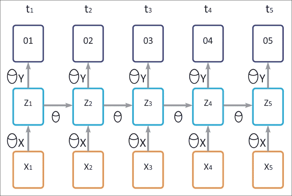  在上圖中，我們有以下參數： * `θ`表示隱藏的循環層的參數 * `θ[x]`表示隱藏層的輸入參數 * `θ[y]`表示輸出層的參數 * `σ`表示隱藏層的激活函數 * 輸入表示為`X[t]` * 隱藏層的輸出為`h[t]` * 最終輸出為`o[t]` * `t`（時間步長） 注意，上圖表示下面給出的循環神經網絡模型的時間流逝。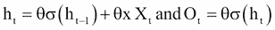現在，如果你回憶一下圖 1，輸出可以表示如下：  現在讓`E`代表輸出層的損失：`E = f(O[t])`。然后，上述三個方程告訴我們`E`取決于輸出`O[t]`。輸出`O[t]`相對于層的隱藏狀態（`h[t]`）的變化而變化。當前時間步長（`h[t]`）的隱藏狀態取決于先前時間步長（`h[t-1]`）的神經元狀態。現在，下面的等式將清除這個概念。 相對于為隱藏層選擇的參數的損失變化率`= ?E/?θ`，這是一個可以表述如下的鏈規則：  （I） 在前面的等式中，項`?h[t]/?h[k]`不僅有趣而且有用。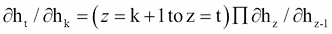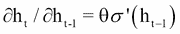  （II） 現在，讓我們考慮`t = 5`和`k = 1`然后  （III） 微分方程（II）相對于（`h[t-1]`）給出了：  （IV） 現在，如果我們將方程（III）和（IV）結合起來，我們可以得到以下結果：  在這些情況下，`θ`也隨著時間步長而變化。上面的等式顯示了當前狀態相對于先前狀態的依賴性。現在讓我們解釋這兩個方程的解剖。假設您處于時間步長 5（`t = 5`），那么`k`的范圍從 1 到 5（`k = 1`到 5），這意味著您必須為以下內容計算`k`）：  現在來看上面的每一個等式（II）  而且，它取決于循環層的參數`θ`。如果在訓練期間你的權重變大，那么由于每個時間步長的等式（I）（II）的乘法，它們將會出現梯度爆炸的問題。 為了克服消失或爆炸問題，已經提出了基本 RNN 模型的各種擴展。將在下一節介紹的 LSTM 網絡就是其中之一。 ## LSTM 網絡 一種 RNN 模型是 LSTM。 LSTM 的精確實現細節不在本書的范圍內。 LSTM 是一種特殊的 RNN 架構，最初由 Hochreiter 和 Schmidhuber 于 1997 年構思。 最近在深度學習的背景下重新發現了這種類型的神經網絡，因為它沒有消失梯度的問題，并且提供了出色的結果和表現。基于 LSTM 的網絡是時間序列的預測和分類的理想選擇，并且正在取代許多傳統的深度學習方法。 這個名稱意味著短期模式不會被遺忘。 LSTM 網絡由彼此鏈接的單元（LSTM 塊）組成。每個 LSTM 塊包含三種類型的門：輸入門，輸出門和遺忘門，它們分別實現對單元存儲器的寫入，讀取和復位功能。這些門不是二元的，而是模擬的（通常由映射在`[0, 1]`范圍內的 Sigmoid 激活函數管理，其中 0 表示總抑制，1 表示總激活）。 如果你認為 LSTM 單元是一個黑盒子，它可以像基本單元一樣使用，除了它會表現得更好；訓練將更快地收斂，它將檢測數據中的長期依賴性。在 TensorFlow 中，您只需使用`BasicLSTMCell`代替`BasicRNNCell`： ```py lstm_cell = tf.nn.rnn_cell.BasicLSTMCell(num_units=n_neurons) ``` LSTM 單元管理兩個狀態向量，并且出于表現原因，它們默認保持獨立。您可以通過在創建`BasicLSTMCell`時設置`state_is_tuple=False`來更改此默認行為。那么，LSTM 單元如何工作？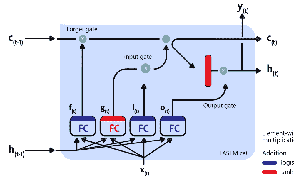基本 LSTM 單元的架構如下圖所示：  圖 11：LSTM 單元的框圖 現在，讓我們看看這個架構背后的數學符號。如果我們不查看 LSTM 框內的內容，LSTM 單元本身看起來就像常規存儲單元，除了它的狀態被分成兩個向量，`h(t)`和`c(t)`： * `h(t)`是短期狀態 * `c(t)`是長期狀態 現在，讓我們打開盒子吧！關鍵的想法是網絡可以學習以下內容： * 在長期的狀態中存儲什么 * 扔掉什么 * 怎么讀它 由于長期`c(t)`從左到右穿過網絡，你可以看到它首先通過一個遺忘門，丟棄一些內存，然后它添加一些新的存儲器通過加法運算（增加了輸入門選擇的存儲器）。結果`c(t)`直接發送，沒有任何進一步的變換 因此，在每個時間步驟，都會丟棄一些內存并添加一些內存。此外，在加法運算之后，長期狀態被復制并通過 tanh 函數，該函數產生`[-1, +1]`范圍內的輸出。 然后輸出門過濾結果。這會產生短期`h(t)`（等于此時間步的單元輸出`y(t)`）。現在，讓我們來看看新記憶的來源以及大門如何運作。首先，當前輸入`x(t)`和之前的短路`h(t-1)`被饋送到四個不同的完全連接。這些門的存在允許 LSTM 單元無限期地記住信息：事實上，如果輸入門低于激活閾值，單元格將保持先前的狀態，如果啟用當前狀態，它將與輸入值組合。顧名思義，遺忘門重置單元的當前狀態（當其值被清除為 0 時），輸出門決定是否必須執行單元的值。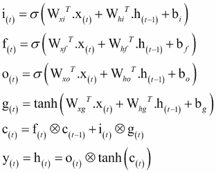 以下等式用于對單個實例的單元的長期狀態，其短期狀態及其在每個時間步的輸出進行 LSTM 計算：  在前面的方程中，`W[xi]`，`W[xf]`，`W[xo]`和`W[xg]`是四個層中每個層的權重矩陣，用于與輸入向量`x(t)`連接。另一方面，`W[hi]`，`W[hf]`，`W[ho]`，和`W[hg]`是四層中每一層的權重矩陣，它們與先前的短期狀態有關。`b[i]`、`b[f]`、`b[o]`、`b[g]`是四層中每一層的偏差項。 TensorFlow 初始化它們為一個全 1 的向量而不是全 0 的向量。這可以防止它在訓練開始時遺忘一切。 ## GRU 單元 LSTM 單元還有許多其他變體。一種特別流行的變體是門控循環單元（GRU）。 Kyunghyun Cho 和其他人在 2014 年的論文中提出了 GRU 單元，該論文還介紹了我們前面提到的自編碼器網絡。 從技術上講，GRU 單元是 LSTM 單元的簡化版本，其中兩個狀態向量合并為一個稱為`h(t)`的向量。單個門控制器控制遺忘門和輸入門。如果門控制器的輸出為 1，則輸入門打開并且遺忘門關閉。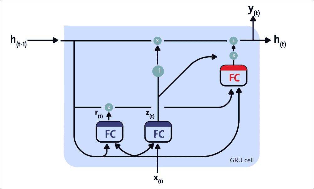  圖 12：GRU 單元 另一方面，如果輸出為 0，則相反。每當必須存儲存儲器時，首先擦除存儲它的位置，這實際上是 LSTM 單元本身的常見變體。第二種簡化是因為在每個時間步輸出滿狀態向量，所以沒有輸出門。但是，新的門控制器控制先前狀態的哪一部分將顯示給主層。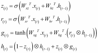 以下等式用于為單個實例，在每個時間步計算 GRU 單元的長期狀態，其短期狀態及其輸出的：  在 TensorFlow 中創建 GRU 單元非常簡單。這是一個例子： ```py gru_cell = tf.nn.rnn_cell.GRUCell(num_units=n_neurons) ``` 這些簡化并不是這種架構的弱點；它似乎成功地執行。 LSTM 或 GRU 單元是近年來 RNN 成功背后的主要原因之一，特別是在 NLP 中的應用。 我們將在本章中看到使用 LSTM 的示例，但下一節將介紹使用 RNN 進行垃圾郵件/火腿文本分類的示例。 # 實現 RNN 進行垃圾郵件預測 在本節中，我們將看到如何在 TensorFlow 中實現 RNN 來預測文本中的垃圾郵件。 ## 數據描述和預處理 將使用來自 UCI ML 倉庫的流行垃圾數據集，可從[此鏈接](http://archive.ics.uci.edu/ml/machine-learning-databases/00228/smssp)下載`amcollection.zip`。 該數據集包含來自多個電子郵件的文本，其中一些被標記為垃圾郵件。在這里，我們將訓練一個模型，該模型將學習僅使用電子郵件文本區分垃圾郵件和非垃圾郵件。讓我們開始導入所需的庫和模型： ```py import os import re import io import requests import numpy as np import matplotlib.pyplot as plt import tensorflow as tf from zipfile import ZipFile from tensorflow.python.framework import ops import warnings ``` 另外，如果您需要，我們可以停止打印由 TensorFlow 產生的警告： ```py warnings.filterwarnings("ignore") os.environ['TF_CPP_MIN_LOG_LEVEL'] = '3' ops.reset_default_graph() ``` 現在，讓我們為圖創建 TensorFlow 會話： ```py sess = tf.Session() ``` 下一個任務是設置 RNN 參數： ```py epochs = 300 batch_size = 250 max_sequence_length = 25 rnn_size = 10 embedding_size = 50 min_word_frequency = 10 learning_rate = 0.0001 dropout_keep_prob = tf.placeholder(tf.float32) ``` 讓我們手動下載數據集并將其存儲在`temp`目錄的`text_data.txt`文件中。首先，我們設置路徑： ```py data_dir = 'temp' data_file = 'text_data.txt' if not os.path.exists(data_dir): os.makedirs(data_dir) ``` 現在，我們直接以壓縮格式下載數據集： ```py if not os.path.isfile(os.path.join(data_dir, data_file)): zip_url = 'http://archive.ics.uci.edu/ml/machine-learning-databases/00228/smsspamcollection.zip' r = requests.get(zip_url) z = ZipFile(io.BytesIO(r.content)) file = z.read('SMSSpamCollection') ``` 我們仍然需要格式化數據： ```py text_data = file.decode() text_data = text_data.encode('ascii',errors='ignore') text_data = text_data.decode().split('\n') ``` 現在，在文本文件中存儲前面提到的目錄： ```py with open(os.path.join(data_dir, data_file), 'w') as file_conn: for text in text_data: file_conn.write("{}\n".format(text)) else: text_data = [] with open(os.path.join(data_dir, data_file), 'r') as file_conn: for row in file_conn: text_data.append(row) text_data = text_data[:-1] ``` 讓我們分開單詞長度至少為 2 的單詞： ```py text_data = [x.split('\t') for x in text_data if len(x)>=1] [text_data_target, text_data_train] = [list(x) for x in zip(*text_data)] ``` 現在我們創建一個文本清理函數： ```py def clean_text(text_string): text_string = re.sub(r'([^\s\w]|_|[0-9])+', '', text_string) text_string = " ".join(text_string.split()) text_string = text_string.lower() return(text_string) ``` 我們調用前面的方法來清理文本： ```py text_data_train = [clean_text(x) for x in text_data_train] ``` 現在我們需要做一個最重要的任務，即創建單詞嵌入 - 將文本更改為數字向量： ```py vocab_processor = tf.contrib.learn.preprocessing.VocabularyProcessor(max_sequence_length, min_frequency=min_word_frequency) text_processed = np.array(list(vocab_processor.fit_transform(text_data_train))) ``` 現在讓我們隨意改變數據集的平衡： ```py text_processed = np.array(text_processed) text_data_target = np.array([1 if x=='ham' else 0 for x in text_data_target]) shuffled_ix = np.random.permutation(np.arange(len(text_data_target))) x_shuffled = text_processed[shuffled_ix] y_shuffled = text_data_target[shuffled_ix] ``` 現在我們已經改組了數據，我們可以將數據分成訓練和測試集： ```py ix_cutoff = int(len(y_shuffled)*0.75) x_train, x_test = x_shuffled[:ix_cutoff], x_shuffled[ix_cutoff:] y_train, y_test = y_shuffled[:ix_cutoff], y_shuffled[ix_cutoff:] vocab_size = len(vocab_processor.vocabulary_) print("Vocabulary size: {:d}".format(vocab_size)) print("Training set size: {:d}".format(len(y_train))) print("Test set size: {:d}".format(len(y_test))) ``` 以下是上述代碼的輸出： ```py >>> Vocabulary size: 933 Training set size: 4180 Test set size: 1394 ``` 在我們開始訓練之前，讓我們為 TensorFlow 圖創建占位符： ```py x_data = tf.placeholder(tf.int32, [None, max_sequence_length]) y_output = tf.placeholder(tf.int32, [None]) ``` 讓我們創建嵌入： ```py embedding_mat = tf.get_variable("embedding_mat", shape=[vocab_size, embedding_size], dtype=tf.float32, initializer=None, regularizer=None, trainable=True, collections=None) embedding_output = tf.nn.embedding_lookup(embedding_mat, x_data) ``` 現在是構建我們的 RNN 的時候了。以下代碼定義了 RNN 單元： ```py cell = tf.nn.rnn_cell.BasicRNNCell(num_units = rnn_size) output, state = tf.nn.dynamic_rnn(cell, embedding_output, dtype=tf.float32) output = tf.nn.dropout(output, dropout_keep_prob) ``` 現在讓我們定義從 RNN 序列獲取輸出的方法： ```py output = tf.transpose(output, [1, 0, 2]) last = tf.gather(output, int(output.get_shape()[0]) - 1) ``` 接下來，我們定義 RNN 的權重和偏置： ```py weight = bias = tf.get_variable("weight", shape=[rnn_size, 2], dtype=tf.float32, initializer=None, regularizer=None, trainable=True, collections=None) bias = tf.get_variable("bias", shape=[2], dtype=tf.float32, initializer=None, regularizer=None, trainable=True, collections=None) ``` 然后定義`logits`輸出。它使用前面代碼中的權重和偏置： ```py logits_out = tf.nn.softmax(tf.matmul(last, weight) + bias) ``` 現在我們定義每個預測的損失，以便稍后，它們可以為損失函數做出貢獻： ```py losses = tf.nn.sparse_softmax_cross_entropy_with_logits_v2(logits=logits_out, labels=y_output) ``` 然后我們定義損失函數： ```py loss = tf.reduce_mean(losses) ``` 我們現在定義每個預測的準確率： ```py accuracy = tf.reduce_mean(tf.cast(tf.equal(tf.argmax(logits_out, 1), tf.cast(y_output, tf.int64)), tf.float32)) ``` 然后我們用`RMSPropOptimizer`創建`training_op`： ```py optimizer = tf.train.RMSPropOptimizer(learning_rate) train_step = optimizer.minimize(loss) ``` 現在讓我們使用`global_variables_initializer()`方法初始化所有變量 ： ```py init_op = tf.global_variables_initializer() sess.run(init_op) ``` 此外，我們可以創建一些空列表來跟蹤每個周期的訓練損失，測試損失，訓練準確率和測試準確率： ```py train_loss = [] test_loss = [] train_accuracy = [] test_accuracy = [] ``` 現在我們已準備好進行訓練，讓我們開始吧。訓練的工作流程如下： * 打亂訓練數據 * 選擇訓練集并計算周期 * 為每個批次運行訓練步驟 * 運行損失和訓練的準確率 * 運行評估步驟。 以下代碼包括上述所有步驟： ```py shuffled_ix = np.random.permutation(np.arange(len(x_train))) x_train = x_train[shuffled_ix] y_train = y_train[shuffled_ix] num_batches = int(len(x_train)/batch_size) + 1 for i in range(num_batches): min_ix = i * batch_size max_ix = np.min([len(x_train), ((i+1) * batch_size)]) x_train_batch = x_train[min_ix:max_ix] y_train_batch = y_train[min_ix:max_ix] train_dict = {x_data: x_train_batch, y_output: \ y_train_batch, dropout_keep_prob:0.5} sess.run(train_step, feed_dict=train_dict) temp_train_loss, temp_train_acc = sess.run([loss,\ accuracy], feed_dict=train_dict) train_loss.append(temp_train_loss) train_accuracy.append(temp_train_acc) test_dict = {x_data: x_test, y_output: y_test, \ dropout_keep_prob:1.0} temp_test_loss, temp_test_acc = sess.run([loss, accuracy], \ feed_dict=test_dict) test_loss.append(temp_test_loss) test_accuracy.append(temp_test_acc) print('Epoch: {}, Test Loss: {:.2}, Test Acc: {:.2}'.format(epoch+1, temp_test_loss, temp_test_acc)) print('\nOverall accuracy on test set (%): {}'.format(np.mean(temp_test_acc)*100.0)) ``` 以下是前面代碼的輸出： ```py >>> Epoch: 1, Test Loss: 0.68, Test Acc: 0.82 Epoch: 2, Test Loss: 0.68, Test Acc: 0.82 Epoch: 3, Test Loss: 0.67, Test Acc: 0.82 … Epoch: 997, Test Loss: 0.36, Test Acc: 0.96 Epoch: 998, Test Loss: 0.36, Test Acc: 0.96 Epoch: 999, Test Loss: 0.35, Test Acc: 0.96 Epoch: 1000, Test Loss: 0.35, Test Acc: 0.96 Overall accuracy on test set (%): 96.19799256324768 ``` 做得好！ RNN 的準確率高于 96%，非常出色。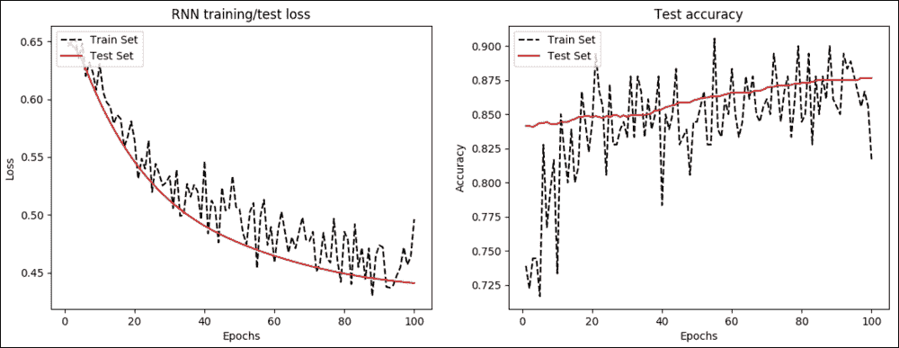現在讓我們觀察損失如何在每次迭代中傳播并隨著時間的推移： ```py epoch_seq = np.arange(1, epochs+1) plt.plot(epoch_seq, train_loss, 'k--', label='Train Set') plt.plot(epoch_seq, test_loss, 'r-', label='Test Set') plt.title('RNN training/test loss') plt.xlabel('Epochs') plt.ylabel('Loss') plt.legend(loc='upper left') plt.show() ```  圖 13：a）每個周期的 RNN 訓練和測試損失 b）每個周期的測試精度 我們還隨時間繪制準確率： ```py plt.plot(epoch_seq, train_accuracy, 'k--', label='Train Set') plt.plot(epoch_seq, test_accuracy, 'r-', label='Test Set') plt.title('Test accuracy') plt.xlabel('Epochs') plt.ylabel('Accuracy') plt.legend(loc='upper left') plt.show() ``` 下一個應用使用時間序列數據進行預測建模。我們還將看到如何開發更復雜的 RNN，稱為 LSTM 網絡。 # 開發時間序列數據的預測模型 RNN，特別是 LSTM 模型，通常是一個難以理解的主題。由于數據中的時間依賴性，時間序列預測是 RNN 的有用應用。時間序列數據可在線獲取。在本節中，我們將看到使用 LSTM 處理時間序列數據的示例。我們的 LSTM 網絡將能夠預測未來的航空公司乘客數量。 ## 數據集的描述 我將使用的數據集是 1949 年至 1960 年國際航空公司乘客的數據。該數據集可以從[此鏈接](https://datamarket.com/data/set/22u3/international-airlinepassengers- monthly-totals-in#!ds=22u3&display=line)。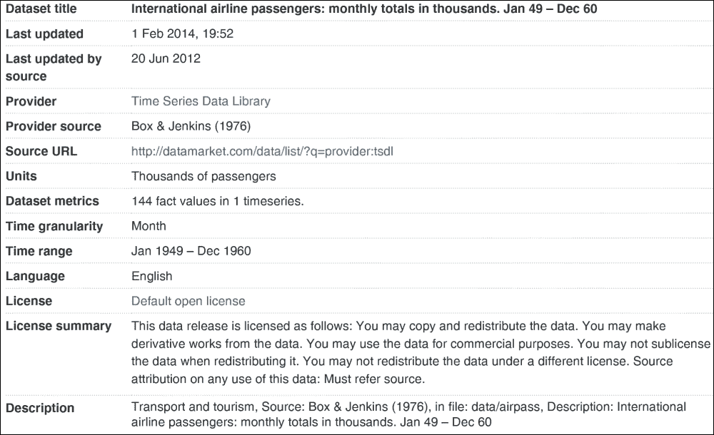以下屏幕截圖顯示了國際航空公司乘客的元數據：  圖 14：國際航空公司乘客的元數據（來源：<https://datamarket.com/>） 您可以通過選擇“導出”選項卡，然后在“導出”組中選擇 CSV 來下載數據。您必須手動編輯 CSV 文件以刪除標題行以及其他頁腳行。我已經下載并保存了名為`international-airline-passengers.csv`的數據文件。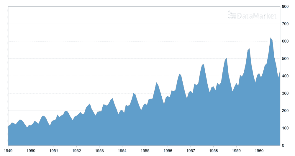下圖是時間序列數據的一個很好的圖：  圖 15：國際航空公司乘客：1 月 49 日至 12 月 60 日的月度總數為千人 ## 預處理和探索性分析 現在讓我們加載原始數據集并查看一些事實。首先，我們加載時間序列如下（見`time_series_preprocessor.py`）： ```py import csv import numpy as np ``` 在這里，我們可以看到`load_series()`的簽名，它是一個用戶定義的方法，可以加載時間序列并對其進行正則化： ```py def load_series(filename, series_idx=1): try: with open(filename) as csvfile: csvreader = csv.reader(csvfile) data = [float(row[series_idx]) for row in csvreader if len(row) > 0] normalized_data = (data - np.mean(data)) / np.std(data) return normalized_data except IOError: Print("Error occurred") return None ``` 現在讓我們調用前面的方法加載時間序列并打印（在終端上發出`$ python3 plot_time_series.py`）數據集中的序列號： ```py import csv import numpy as np import matplotlib.pyplot as plt import time_series_preprocessor as tsp timeseries = tsp.load_series('international-airline-passengers.csv') print(timeseries) ``` 以下是前面代碼的輸出： ```py >>> [-1.40777884 -1.35759023 -1.24048348 -1.26557778 -1.33249593 -1.21538918 -1.10664719 -1.10664719 -1.20702441 -1.34922546 -1.47469699 -1.35759023 ….. 2.85825285 2.72441656 1.9046693 1.5115252 0.91762667 1.26894693] print(np.shape(timeseries)) ``` ```py >>> 144 ``` 這意味著時間序列中有`144`條目。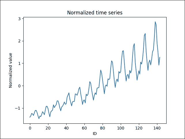讓我們繪制時間序列： ```py plt.figure() plt.plot(timeseries) plt.title('Normalized time series') plt.xlabel('ID') plt.ylabel('Normalized value') plt.legend(loc='upper left') plt.show() ``` 以下是上述代碼的輸出： ```py >>> ```  圖 16：時間序列（y 軸，標準化值與 x 軸，ID） 加載時間序列數據集后，下一個任務是準備訓練集。由于我們將多次評估模型以預測未來值，因此我們將數據分為訓練和測試。更具體地說，`split_data()`函數將數據集劃分為兩個部分，用于訓練和測試，75% 用于訓練，25% 用于測試： ```py def split_data(data, percent_train): num_rows = len(data) train_data, test_data = [], [] for idx, row in enumerate(data): if idx < num_rows * percent_train: train_data.append(row) else: test_data.append(row) return train_data, test_data ``` ## LSTM 預測模型 一旦我們準備好數據集，我們就可以通過以可接受的格式加載數據來訓練預測器。在這一步中，我編寫了一個名為`TimeSeriesPredictor.py`的 Python 腳本，它首先導入必要的庫和模塊（在此腳本的終端上發出`$ python3 TimeSeriesPredictor.py`命令）： ```py import numpy as np import tensorflow as tf from tensorflow.python.ops import rnn, rnn_cell import time_series_preprocessor as tsp import matplotlib.pyplot as plt ``` 接下來，我們為 LSTM 網絡定義超參數（相應地調整它）： ```py input_dim = 1 seq_size = 5 hidden_dim = 5 ``` 我們現在定義權重變量（無偏差）和輸入占位符： ```py W_out = tf.get_variable("W_out", shape=[hidden_dim, 1], dtype=tf.float32, initializer=None, regularizer=None, trainable=True, collections=None) b_out = tf.get_variable("b_out", shape=[1], dtype=tf.float32, initializer=None, regularizer=None, trainable=True, collections=None) x = tf.placeholder(tf.float32, [None, seq_size, input_dim]) y = tf.placeholder(tf.float32, [None, seq_size]) ``` 下一個任務是構建 LSTM 網絡。以下方法`LSTM_Model()`采用三個參數，如下所示： * `x`：大小為`[T, batch_size, input_size]`的輸入 * `W`：完全連接的輸出層權重矩陣 * `b`：完全連接的輸出層偏置向量 現在讓我們看一下方法的簽名： ```py def LSTM_Model(): cell = rnn_cell.BasicLSTMCell(hidden_dim) outputs, states = rnn.dynamic_rnn(cell, x, dtype=tf.float32) num_examples = tf.shape(x)[0] W_repeated = tf.tile(tf.expand_dims(W_out, 0), [num_examples, 1, 1]) out = tf.matmul(outputs, W_repeated) + b_out out = tf.squeeze(out) return out ``` 此外，我們創建了三個空列表來存儲訓練損失，測試損失和步驟： ```py train_loss = [] test_loss = [] step_list = [] ``` 下一個名為`train()`的方法用于訓練 LSTM 網絡： ```py def trainNetwork(train_x, train_y, test_x, test_y): with tf.Session() as sess: tf.get_variable_scope().reuse_variables() sess.run(tf.global_variables_initializer()) max_patience = 3 patience = max_patience min_test_err = float('inf') step = 0 while patience > 0: _, train_err = sess.run([train_op, cost], feed_dict={x: train_x, y: train_y}) if step % 100 == 0: test_err = sess.run(cost, feed_dict={x: test_x, y: test_y}) print('step: {}\t\ttrain err: {}\t\ttest err: {}'.format(step, train_err, test_err)) train_loss.append(train_err) test_loss.append(test_err) step_list.append(step) if test_err < min_test_err: min_test_err = test_err patience = max_patience else: patience -= 1 step += 1 save_path = saver.save(sess, 'model.ckpt') print('Model saved to {}'.format(save_path)) ``` 接下來的任務是創建成本優化器并實例化`training_op`： ```py cost = tf.reduce_mean(tf.square(LSTM_Model()- y)) train_op = tf.train.AdamOptimizer(learning_rate=0.003).minimize(cost) ``` 另外，這里有一個叫做保存模型的輔助`op`： ```py saver = tf.train.Saver() ``` 現在我們已經創建了模型，下一個方法稱為`testLSTM()`，用于測試模型在測試集上的預測能力： ```py def testLSTM(sess, test_x): tf.get_variable_scope().reuse_variables() saver.restore(sess, 'model.ckpt') output = sess.run(LSTM_Model(), feed_dict={x: test_x}) return output ``` 為了繪制預測結果，我們有一個名為`plot_results()`的函數。簽名如下： ```py def plot_results(train_x, predictions, actual, filename): plt.figure() num_train = len(train_x) plt.plot(list(range(num_train)), train_x, color='b', label='training data') plt.plot(list(range(num_train, num_train + len(predictions))), predictions, color='r', label='predicted') plt.plot(list(range(num_train, num_train + len(actual))), actual, color='g', label='test data') plt.legend() if filename is not None: plt.savefig(filename) else: plt.show() ``` ## 模型評估 為了評估模型，我們有一個名為`main()`的方法，它實際上調用前面的方法來創建和訓練 LSTM 網絡。代碼的工作流程如下： 1. 加載數據 2. 在時間序列數據中滑動窗口以構建訓練數據集 3. 執行相同的窗口滑動策略來構建測試數據集 4. 在訓練數據集上訓練模型 5. 可視化模型的表現 讓我們看看方法的簽名： ```py def main(): data = tsp.load_series('international-airline-passengers.csv') train_data, actual_vals = tsp.split_data(data=data, percent_train=0.75) train_x, train_y = [], [] for i in range(len(train_data) - seq_size - 1): train_x.append(np.expand_dims(train_data[i:i+seq_size], axis=1).tolist()) train_y.append(train_data[i+1:i+seq_size+1]) test_x, test_y = [], [] for i in range(len(actual_vals) - seq_size - 1): test_x.append(np.expand_dims(actual_vals[i:i+seq_size], axis=1).tolist()) test_y.append(actual_vals[i+1:i+seq_size+1]) trainNetwork(train_x, train_y, test_x, test_y) with tf.Session() as sess: predicted_vals = testLSTM(sess, test_x)[:,0] # Following prediction results of the model given ground truth values plot_results(train_data, predicted_vals, actual_vals, 'ground_truth_predition.png') prev_seq = train_x[-1] predicted_vals = [] for i in range(1000): next_seq = testLSTM(sess, [prev_seq]) predicted_vals.append(next_seq[-1]) prev_seq = np.vstack((prev_seq[1:], next_seq[-1])) # Following predictions results where only the training data was given plot_results(train_data, predicted_vals, actual_vals, 'prediction_on_train_set.png') >>> ``` 最后，我們將調用`main()`方法來執行訓練。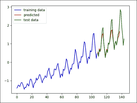訓練完成后，它進一步繪制模型的預測結果，包括地面實況值與預測結果，其中只給出了訓練數據： ```py >>> ```  圖 17：模型對地面實況值的結果 下圖顯示了訓練數據的預測結果。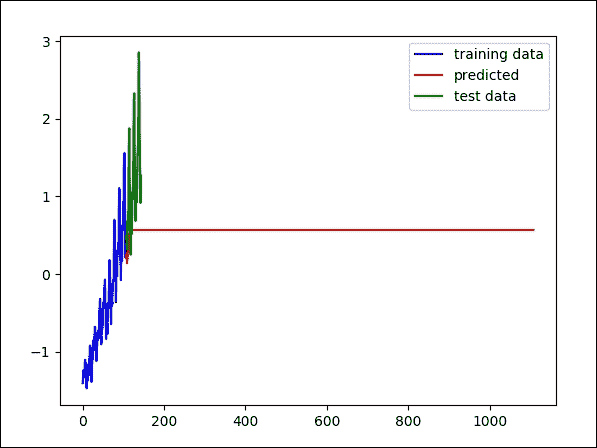此過程可用的信息較少，但它仍然可以很好地匹配數據中的趨勢：  圖 18：訓練集上模型的結果 以下方法幫助我們繪制訓練和測試誤差： ```py def plot_error(): # Plot training loss over time plt.plot(step_list, train_loss, 'r--', label='LSTM training loss per iteration', linewidth=4) plt.title('LSTM training loss per iteration') plt.xlabel('Iteration') plt.ylabel('Training loss') plt.legend(loc='upper right') plt.show() # Plot test loss over time plt.plot(step_list, test_loss, 'r--', label='LSTM test loss per iteration', linewidth=4) plt.title('LSTM test loss per iteration') plt.xlabel('Iteration') plt.ylabel('Test loss') plt.legend(loc='upper left') plt.show() ``` 現在我們調用上面的方法如下： ```py plot_error() >>> ```  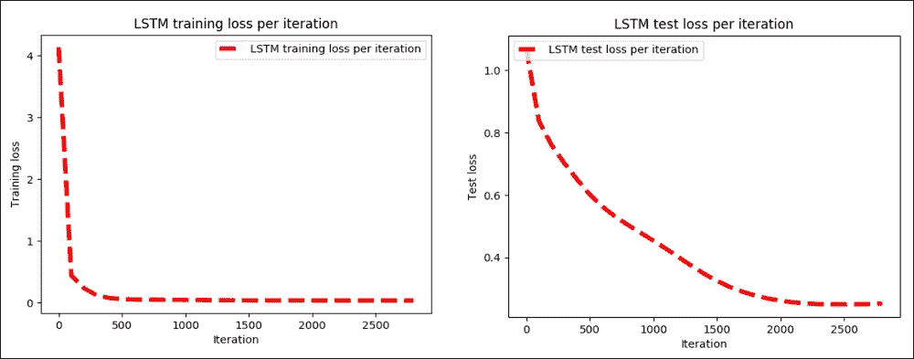圖 19：a）每次迭代的 LSTM 訓練損失，b）每次迭代的 LSTM 測試損失 我們可以使用時間序列預測器來重現數據中的實際波動。現在，您可以準備自己的數據集并執行其他一些預測分析。下一個示例是關于產品和電影評論數據集的情感分析。我們還將了解如何使用 LSTM 網絡開發更復雜的 RNN。 # 用于情感分析的 LSTM 預測模型 情感分析是 NLP 中使用最廣泛的任務之一。 LSTM 網絡可用于將短文本分類為期望的類別，即分類問題。例如，一組推文可以分為正面或負面。在本節中，我們將看到這樣一個例子。 ## 網絡設計 實現的 LSTM 網絡將具有三層：嵌入層，RNN 層和 softmax 層。從下圖可以看到對此的高級視圖。在這里，我總結了所有層的功能： * 嵌入層：我們將在第 8 章中看到一個示例，顯示文本數據集不能直接饋送到深度神經網絡（DNN），因此一個名為嵌入層是必需的。對于該層，我們將每個輸入（k 個單詞的張量）變換為 k 個 N 維向量的張量。這稱為字嵌入，其中 N 是嵌入大小。每個單詞都與在訓練過程中需要學習的權重向量相關聯。您可以在單詞的向量表示中更深入地了解單詞嵌入。 * RNN 層：一旦我們構建了嵌入層，就會有一個名為 RNN 層的新層，它由帶有壓降包裝的 LSTM 單元組成。在訓練過程中需要學習 LSTM 權重，如前幾節所述。動態展開 RNN 層（如圖 4 所示），將 k 個字嵌入作為輸入并輸出 k 個 M 維向量，其中 M 是 LSTM 單元的隱藏大小。 * Softmax 或 Sigmoid 層：RNN 層的輸出在`k`個時間步長上平均，獲得大小為`M`的單個張量。最后，例如，softmax 層用于計算分類概率。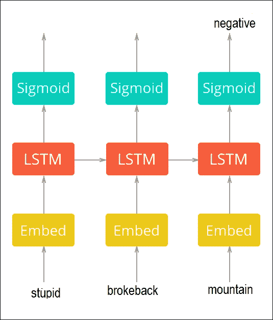  圖 20：用于情感分析的 LSTM 網絡的高級視圖 稍后我們將看到交叉熵如何用作損失函數，`RMSProp`是最小化它的優化器。 ## LSTM 模型訓練 UMICH SI650 - 情感分類數據集（刪除了重復）包含有關密歇根大學捐贈的產品和電影評論的數據，可以從[此鏈接下載](https://inclass.kaggle.com/c/si650winter11/data/)。在獲取令牌之前，已經清除了不需要的或特殊的字符（參見`data.csv`文件）。 以下腳本還會刪除停用詞（請參閱`data_preparation.py`）。給出一些標記為陰性或陽性的樣本（1 為正面，0 為負面）： | 情感 | 情感文本 | | --- | --- | | 1 | 達芬奇密碼書真棒。 | | 1 | 我很喜歡達芬奇密碼。 | | 0 | 天哪，我討厭斷背山。 | | 0 | 我討厭哈利波特。 | > 表 1：情感數據集的樣本 現在，讓我們看一下為此任務訓練 LSTM 網絡的分步示例。首先，我們導入必要的模塊和包（執行`train.py`文件）： ```py from data_preparation import Preprocessing from lstm_network import LSTM_RNN_Network import tensorflow as tf import pickle import datetime import time import os import matplotlib.pyplot as plt ``` 在前面的導入聲明中，`data_preparation`和`lstm_network`是兩個輔助 Python 腳本，用于數據集準備和網絡設計。我們稍后會看到更多細節。現在讓我們為 LSTM 定義參數： ```py data_dir = 'data/' # Data directory containing 'data.csv' stopwords_file = 'data/stopwords.txt' # Path to stopwords file n_samples= None # Set n_samples=None to use the whole dataset # Directory where TensorFlow summaries will be stored' summaries_dir= 'logs/' batch_size = 100 #Batch size train_steps = 1000 #Number of training steps hidden_size= 75 # Hidden size of LSTM layer embedding_size = 75 # Size of embeddings layer learning_rate = 0.01 test_size = 0.2 dropout_keep_prob = 0.5 # Dropout keep-probability sequence_len = None # Maximum sequence length validate_every = 100 # Step frequency to validate ``` 我相信前面的參數是不言自明的。下一個任務是準備 TensorBoard 使用的摘要： ```py summaries_dir = '{0}/{1}'.format(summaries_dir, datetime.datetime.now().strftime('%d_%b_%Y-%H_%M_%S')) train_writer = tf.summary.FileWriter(summaries_dir + '/train') validation_writer = tf.summary.FileWriter(summaries_dir + '/validation') ``` 現在讓我們準備模型目錄： ```py model_name = str(int(time.time())) model_dir = '{0}/{1}'.format(checkpoints_root, model_name) if not os.path.exists(model_dir): os.makedirs(model_dir) ``` 接下來，讓我們準備數據并構建 TensorFlow 圖（參見`data_preparation.py`文件）： ```py data_lstm = Preprocessing(data_dir=data_dir, stopwords_file=stopwords_file, sequence_len=sequence_len, test_size=test_size, val_samples=batch_size, n_samples=n_samples, random_state=100) ``` 在前面的代碼段中，`Preprocessing`是一個繼續的類（詳見`data_preparation.py`）幾個函數和構造器，它們幫助我們預處理訓練和測試集以訓練 LSTM 網絡。在這里，我提供了每個函數及其功能的代碼。 該類的構造器初始化數據預處理器。此類提供了一個接口，用于將數據加載，預處理和拆分為訓練，驗證和測試集。它需要以下參數： * `data_dir`：包含數據集文件`data.csv`的數據目錄，其中包含名為`SentimentText`和`Sentiment`的列。 * `stopwords_file`：可選。如果提供，它將丟棄原始數據中的每個停用詞。 * `sequence_len`：可選。如果`m`是數據集中的最大序列長度，則需要`sequence_len >= m`。如果`sequence_len`為`None`，則會自動分配給`m`。 * `n_samples`：可選。它是從數據集加載的樣本數（對大型數據集很有用）。如果`n_samples`是`None`，則將加載整個數據集（注意；如果數據集很大，則可能需要一段時間來預處理每個樣本）。 * `test_size`：可選。`0 < test_size < 1`。它表示要包含在測試集中的數據集的比例（默認值為`0.2`）。 * `val_samples`：可選但可用于表示驗證樣本的絕對數量（默認為`100`）。 * `random_state`：這是隨機種子的可選參數，用于將數據分成訓練，測試和驗證集（默認為`0`）。 * `ensure_preprocessed`：可選。如果`ensure_preprocessed=True`，它確保數據集已經過預處理（默認為`False`）。 構造器的代碼如下： ```py def __init__(self, data_dir, stopwords_file=None, sequence_len=None, n_samples=None, test_size=0.2, val_samples=100, random_state=0, ensure_preprocessed=False): self._stopwords_file = stopwords_file self._n_samples = n_samples self.sequence_len = sequence_len self._input_file = os.path.join(data_dir, 'data.csv') self._preprocessed_file=os.path.join(data_dir,"preprocessed_"+str(n_samples)+ ".npz") self._vocab_file = os.path.join(data_dir,"vocab_" + str(n_samples) + ".pkl") self._tensors = None self._sentiments = None self._lengths = None self._vocab = None self.vocab_size = None # Prepare data if os.path.exists(self._preprocessed_file)and os.path.exists(self._vocab_file): print('Loading preprocessed files ...') self.__load_preprocessed() else: if ensure_preprocessed: raise ValueError('Unable to findpreprocessed files.') print('Reading data ...') self.__preprocess() # Split data in train, validation and test sets indices = np.arange(len(self._sentiments)) x_tv, self._x_test, y_tv, self._y_test,tv_indices, test_indices = train_test_split( self._tensors, self._sentiments, indices, test_size=test_size, random_state=random_state, stratify=self._sentiments[:, 0]) self._x_train,self._x_val,self._y_train,self._y_val,train_indices,val_indices= train_test_split(x_tv, y_tv, tv_indices, test_size=val_samples,random_state = random_state, stratify=y_tv[:, 0]) self._val_indices = val_indices self._test_indices = test_indices self._train_lengths = self._lengths[train_indices] self._val_lengths = self._lengths[val_indices] self._test_lengths = self._lengths[test_indices] self._current_index = 0 self._epoch_completed = 0 ``` 現在讓我們看看前面方法的簽名。我們從`_preprocess()`方法開始，該方法從`data_dir` / `data.csv`加載數據，預處理每個加載的樣本，并存儲中間文件以避免以后進行預處理。工作流程如下： 1. 加載數據 2. 清理示例文本 3. 準備詞匯詞典 4. 刪除最不常見的單詞（它們可能是語法錯誤），將樣本編碼為張量，并根據`sequence_len`用零填充每個張量 5. 保存中間文件 6. 存儲樣本長度以備將來使用 現在讓我們看看下面的代碼塊，它代表了前面的工作流程： ```py def __preprocess(self): data = pd.read_csv(self._input_file, nrows=self._n_samples) self._sentiments = np.squeeze(data.as_matrix(columns=['Sentiment'])) self._sentiments = np.eye(2)[self._sentiments] samples = data.as_matrix(columns=['SentimentText'])[:, 0] samples = self.__clean_samples(samples) vocab = dict() vocab[''] = (0, len(samples)) # add empty word for sample in samples: sample_words = sample.split() for word in list(set(sample_words)): # distinct words value = vocab.get(word) if value is None: vocab[word] = (-1, 1) else: encoding, count = value vocab[word] = (-1, count + 1) sample_lengths = [] tensors = [] word_count = 1 for sample in samples: sample_words = sample.split() encoded_sample = [] for word in list(set(sample_words)): # distinct words value = vocab.get(word) if value is not None: encoding, count = value if count / len(samples) > 0.0001: if encoding == -1: encoding = word_count vocab[word] = (encoding, count) word_count += 1 encoded_sample += [encoding] else: del vocab[word] tensors += [encoded_sample] sample_lengths += [len(encoded_sample)] self.vocab_size = len(vocab) self._vocab = vocab self._lengths = np.array(sample_lengths) self.sequence_len, self._tensors = self.__apply_to_zeros(tensors, self.sequence_len) with open(self._vocab_file, 'wb') as f: pickle.dump(self._vocab, f) np.savez(self._preprocessed_file, tensors=self._tensors, lengths=self._lengths, sentiments=self._sentiments) ``` 接下來，我們調用前面的方法并加載中間文件，避免數據預處理： ```py def __load_preprocessed(self): with open(self._vocab_file, 'rb') as f: self._vocab = pickle.load(f) self.vocab_size = len(self._vocab) load_dict = np.load(self._preprocessed_file) self._lengths = load_dict['lengths'] self._tensors = load_dict['tensors'] self._sentiments = load_dict['sentiments'] self.sequence_len = len(self._tensors[0]) ``` 一旦我們預處理數據集，下一個任務就是清理樣本。工作流程如下： 1. 準備正則表達式模式。 2. 清理每個樣本。 3. 恢復 HTML 字符。 4. 刪除`@users`和 URL。 5. 轉換為小寫。 6. 刪除標點符號。 7. 用`C`替換`C+`（連續出現兩次以上的字符） 8. 刪除停用詞。 現在讓我們以編程方式編寫上述步驟。為此，我們有以下函數： ```py def __clean_samples(self, samples): print('Cleaning samples ...') ret = [] reg_punct = '[' + re.escape(''.join(string.punctuation)) + ']' if self._stopwords_file is not None: stopwords = self.__read_stopwords() sw_pattern = re.compile(r'\b(' + '|'.join(stopwords) + r')\b') for sample in samples: text = html.unescape(sample) words = text.split() words = [word for word in words if not word.startswith('@') and not word.startswith('http://')] text = ' '.join(words) text = text.lower() text = re.sub(reg_punct, ' ', text) text = re.sub(r'([a-z])\1{2,}', r'\1', text) if stopwords is not None: text = sw_pattern.sub('', text) ret += [text] return ret ``` `__apply_to_zeros()`方法返回使用的`padding_length`和填充張量的 NumPy 數組。首先，它找到最大長度`m`，并確保`m>=sequence_len`。然后根據`sequence_len`用零填充列表： ```py def __apply_to_zeros(self, lst, sequence_len=None): inner_max_len = max(map(len, lst)) if sequence_len is not None: if inner_max_len > sequence_len: raise Exception('Error: Provided sequence length is not sufficient') else: inner_max_len = sequence_len result = np.zeros([len(lst), inner_max_len], np.int32) for i, row in enumerate(lst): for j, val in enumerate(row): result[i][j] = val return inner_max_len, result ``` 下一個任務是刪除所有停用詞（在`data` / `StopWords.txt file`中提供）。此方法返回停用詞列表： ```py def __read_stopwords(self): if self._stopwords_file is None: return None with open(self._stopwords_file, mode='r') as f: stopwords = f.read().splitlines() return stopwords ``` `next_batch()`方法將`batch_size>0`作為包含的樣本數，在完成周期后返回批量大小樣本（`text_tensor`，`text_target`，`text_length`），并隨機抽取訓練樣本： ```py def next_batch(self, batch_size): start = self._current_index self._current_index += batch_size if self._current_index > len(self._y_train): self._epoch_completed += 1 ind = np.arange(len(self._y_train)) np.random.shuffle(ind) self._x_train = self._x_train[ind] self._y_train = self._y_train[ind] self._train_lengths = self._train_lengths[ind] start = 0 self._current_index = batch_size end = self._current_index return self._x_train[start:end], self._y_train[start:end], self._train_lengths[start:end] ``` 然后使用稱為`get_val_data()`的下一個方法來獲取在訓練期間使用的驗證集。它接受原始文本并返回驗證數據。默認情況下，它返回`original_text`（`original_samples`，`text_tensor`，`text_target`，`text_length`），否則返回`text_tensor`，`text_target`，`text_length`： ```py def get_val_data(self, original_text=False): if original_text: data = pd.read_csv(self._input_file, nrows=self._n_samples) samples = data.as_matrix(columns=['SentimentText'])[:, 0] return samples[self._val_indices], self._x_val, self._y_val, self._val_lengths return self._x_val, self._y_val, self._val_lengths ``` 最后， 是一個名為`get_test_data()`的附加方法，用于準備將在模型評估期間使用的測試集： ```py def get_test_data(self, original_text=False): if original_text: data = pd.read_csv(self._input_file, nrows=self._n_samples) samples = data.as_matrix(columns=['SentimentText'])[:, 0] return samples[self._test_indices], self._x_test, self._y_test, self._test_lengths return self._x_test, self._y_test, self._test_lengths ``` 現在我們準備數據，以便 LSTM 網絡可以提供它： ```py lstm_model = LSTM_RNN_Network(hidden_size=[hidden_size], vocab_size=data_lstm.vocab_size, embedding_size=embedding_size, max_length=data_lstm.sequence_len, learning_rate=learning_rate) ``` 在前面的代碼段中，`LSTM_RNN_Network`是一個包含多個函數和構造器的類，可幫助我們創建 LSTM 網絡。即將推出的構造器構建了 TensorFlow LSTM 模型。它需要以下參數： * `hidden_size`：一個數組，保存 rnn 層的 LSTM 單元中的單元數 * `vocab_size`：樣本中的詞匯量大小 * `embedding_size`：將使用此大小的向量對單詞進行編碼 * `max_length`：輸入張量的最大長度 * `n_classes`：類別的數量 * `learning_rate`：RMSProp 算法的學習率 * `random_state`：丟棄的隨機狀態 構造器的代碼如下： ```py def __init__(self, hidden_size, vocab_size, embedding_size, max_length, n_classes=2, learning_rate=0.01, random_state=None): # Build TensorFlow graph self.input = self.__input(max_length) self.seq_len = self.__seq_len() self.target = self.__target(n_classes) self.dropout_keep_prob = self.__dropout_keep_prob() self.word_embeddings = self.__word_embeddings(self.input, vocab_size, embedding_size, random_state) self.scores = self.__scores(self.word_embeddings, self.seq_len, hidden_size, n_classes, self.dropout_keep_prob, random_state) self.predict = self.__predict(self.scores) self.losses = self.__losses(self.scores, self.target) self.loss = self.__loss(self.losses) self.train_step = self.__train_step(learning_rate, self.loss) self.accuracy = self.__accuracy(self.predict, self.target) self.merged = tf.summary.merge_all() ``` 下一個函數被稱為`_input()`，它采用一個名為`max_length`的參數，它是輸入張量的最大長度。然后它返回一個輸入占位符，其形狀為`[batch_size, max_length]`，用于 TensorFlow 計算： ```py def __input(self, max_length): return tf.placeholder(tf.int32, [None, max_length], name='input') ``` 接下來，`_seq_len()`函數返回一個形狀為`[batch_size]`的序列長度占位符。它保持給定批次中每個張量的實際長度，允許動態序列長度： ```py def __seq_len(self): return tf.placeholder(tf.int32, [None], name='lengths') ``` 下一個函數稱為`_target()`。它需要一個名為`n_classes`的參數，它包含分類類的數量。最后，它返回形狀為`[batch_size, n_classes]`的目標占位符： ```py def __target(self, n_classes): return tf.placeholder(tf.float32, [None, n_classes], name='target') ``` `_dropout_keep_prob()`返回一個持有丟棄的占位符保持概率以減少過擬合： ```py def __dropout_keep_prob(self): return tf.placeholder(tf.float32, name='dropout_keep_prob') ``` `_cell()`方法用于構建帶有壓差包裝器的 LSTM 單元。它需要以下參數： * `hidden_size`：它是 LSTM 單元中的單元數 * `dropout_keep_prob`：這表示持有丟棄保持概率的張量 * `seed`：它是一個可選值，可確保丟棄包裝器的隨機狀態計算的可重現性。 最后，它返回一個帶有丟棄包裝器的 LSTM 單元： ```py def __cell(self, hidden_size, dropout_keep_prob, seed=None): lstm_cell = tf.nn.rnn_cell.LSTMCell(hidden_size, state_is_tuple=True) dropout_cell = tf.nn.rnn_cell.DropoutWrapper(lstm_cell, input_keep_prob=dropout_keep_prob, output_keep_prob = dropout_keep_prob, seed=seed) return dropout_cell ``` 一旦我們創建了 LSTM 單元格，我們就可以創建輸入標記的嵌入。為此，`__word_embeddings()`可以解決這個問題。它構建一個形狀為`[vocab_size, embedding_size]`的嵌入層，輸入參數如`x`，它是形狀`[batch_size, max_length]`的輸入。`vocab_size`是詞匯量大小，即可能出現在樣本中的可能單詞的數量。`embedding_size`是將使用此大小的向量表示的單詞，種子是可選的，但確保嵌入初始化的隨機狀態。 最后，它返回具有形狀`[batch_size, max_length, embedding_size]`的嵌入查找張量： ```py def __word_embeddings(self, x, vocab_size, embedding_size, seed=None): with tf.name_scope('word_embeddings'): embeddings = tf.get_variable("embeddings",shape=[vocab_size, embedding_size], dtype=tf.float32, initializer=None, regularizer=None, trainable=True, collections=None) embedded_words = tf.nn.embedding_lookup(embeddings, x) return embedded_words ``` `__rnn_layer ()`方法創建 LSTM 層。它需要幾個輸入參數，這里描述： * `hidden_size`：這是 LSTM 單元中的單元數 * `x`：這是帶形狀的輸入 * `seq_len`：這是具有形狀的序列長度張量 * `dropout_keep_prob`：這是持有丟棄保持概率的張量 * `variable_scope`：這是變量范圍的名稱（默認層是`rnn_layer`） * `random_state`：這是丟棄包裝器的隨機狀態 最后，它返回形狀為`[batch_size, max_seq_len, hidden_size]`的輸出： ```py def __rnn_layer(self, hidden_size, x, seq_len, dropout_keep_prob, variable_scope=None, random_state=None): with tf.variable_scope(variable_scope, default_name='rnn_layer'): lstm_cell = self.__cell(hidden_size, dropout_keep_prob, random_state) outputs, _ = tf.nn.dynamic_rnn(lstm_cell, x, dtype=tf.float32, sequence_length=seq_len) return outputs ``` `_score()`方法用于計算網絡輸出。它需要幾個輸入參數，如下所示： * `embedded_words`：這是具有形狀`[batch_size, max_length, embedding_size]`的嵌入查找張量 * `seq_len`：這是形狀`[batch_size]`的序列長度張量 * `hidden_size`：這是一個數組，其中包含每個 RNN 層中 LSTM 單元中的單元數 * `n_classes`：這是類別的數量 * `dropout_keep_prob`：這是持有丟棄保持概率的張量 * `random_state`：這是一個可選參數，但它可用于確保丟棄包裝器的隨機狀態 最后，`_score()`方法返回具有形狀`[batch_size, n_classes]`的每個類的線性激活： ```py def __scores(self, embedded_words, seq_len, hidden_size, n_classes, dropout_keep_prob, random_state=None): outputs = embedded_words for h in hidden_size: outputs = self.__rnn_layer(h, outputs, seq_len, dropout_keep_prob) outputs = tf.reduce_mean(outputs, axis=[1]) with tf.name_scope('final_layer/weights'): w = tf.get_variable("w", shape=[hidden_size[-1], n_classes], dtype=tf.float32, initializer=None, regularizer=None, trainable=True, collections=None) self.variable_summaries(w, 'final_layer/weights') with tf.name_scope('final_layer/biases'): b = tf.get_variable("b", shape=[n_classes], dtype=tf.float32, initializer=None, regularizer=None,trainable=True, collections=None) self.variable_summaries(b, 'final_layer/biases') with tf.name_scope('final_layer/wx_plus_b'): scores = tf.nn.xw_plus_b(outputs, w, b, name='scores') tf.summary.histogram('final_layer/wx_plus_b', scores) return scores ``` `_predict()`方法將得分作為具有形狀`[batch_size, n_classes]`的每個類的線性激活，并以形狀`[batch_size, n_classes]`返回 softmax（以`[0, 1]`的比例標準化得分）激活： ```py def __predict(self, scores): with tf.name_scope('final_layer/softmax'): softmax = tf.nn.softmax(scores, name='predictions') tf.summary.histogram('final_layer/softmax', softmax) return softmax ``` `_losses()`方法返回具有形狀`[batch_size]`的交叉熵損失（因為 softmax 用作激活函數）。它還需要兩個參數，例如得分，作為具有形狀`[batch_size, n_classes]`的每個類的線性激活和具有形狀`[batch_size, n_classes]`的目標張量： ```py def __losses(self, scores, target): with tf.name_scope('cross_entropy'): cross_entropy = tf.nn.softmax_cross_entropy_with_logits_v2(logits=scores, labels=target, name='cross_entropy') return cross_entropy ``` `_loss()`函數計算并返回平均交叉熵損失。它只需要一個參數，稱為損耗，它表示形狀`[batch_size]`的交叉熵損失，并由前一個函數計算： ```py def __loss(self, losses): with tf.name_scope('loss'): loss = tf.reduce_mean(losses, name='loss') tf.summary.scalar('loss', loss) return loss ``` 現在，`_train_step()`計算并返回`RMSProp`訓練步驟操作。它需要兩個參數，`learning_rate`，這是`RMSProp`優化器的學習率；和前一個函數計算的平均交叉熵損失： ```py def __train_step(self, learning_rate, loss): return tf.train.RMSPropOptimizer(learning_rate).minimize(loss) ``` 評估表現時，`_accuracy()`函數計算分類的準確率。它需要三個參數，預測，softmax 激活具有哪種形狀`[batch_size, n_classes]`;和具有形狀`[batch_size, n_classes]`的目標張量和當前批次中獲得的平均精度： ```py def __accuracy(self, predict, target): with tf.name_scope('accuracy'): correct_pred = tf.equal(tf.argmax(predict, 1), tf.argmax(target, 1)) accuracy = tf.reduce_mean(tf.cast(correct_pred, tf.float32), name='accuracy') tf.summary.scalar('accuracy', accuracy) return accuracy ``` 下一個函數被稱為`initialize_all_variable()`，正如您可能猜到的那樣，它初始化所有變量： ```py def initialize_all_variables(self): return tf.global_variables_initializer() ``` 最后，我們有一個名為`variable_summaries()`的靜態方法，它將大量摘要附加到 TensorBoard 可視化的張量上。它需要以下參數： ```py var: is the variable to summarize mean: mean of the summary name. ``` 簽名如下： ```py @staticmethod def variable_summaries(var, name): with tf.name_scope('summaries'): mean = tf.reduce_mean(var) tf.summary.scalar('mean/' + name, mean) with tf.name_scope('stddev'): stddev = tf.sqrt(tf.reduce_mean(tf.square(var - mean))) tf.summary.scalar('stddev/' + name, stddev) tf.summary.scalar('max/' + name, tf.reduce_max(var)) tf.summary.scalar('min/' + name, tf.reduce_min(var)) tf.summary.histogram(name, var) ``` 現在我們需要在訓練模型之前創建一個 TensorFlow 會話： ```py sess = tf.Session() ``` 讓我們初始化所有變量： ```py init_op = tf.global_variables_initializer() sess.run(init_op) ``` 然后我們保存 TensorFlow 模型以備將來使用： ```py saver = tf.train.Saver() ``` 現在讓我們準備訓練集： ```py x_val, y_val, val_seq_len = data_lstm.get_val_data() ``` 現在我們應該編寫 TensorFlow 圖計算的日志： ```py train_writer.add_graph(lstm_model.input.graph) ``` 此外，我們可以創建一些空列表來保存訓練損失，驗證損失和步驟，以便我們以圖形方式查看它們： ```py train_loss_list = [] val_loss_list = [] step_list = [] sub_step_list = [] step = 0 ``` 現在我們開始訓練。在每個步驟中，我們記錄訓練誤差。驗證誤差記錄在每個子步驟中： ```py for i in range(train_steps): x_train, y_train, train_seq_len = data_lstm.next_batch(batch_size) train_loss, _, summary = sess.run([lstm_model.loss, lstm_model.train_step, lstm_model.merged], feed_dict={lstm_model.input: x_train, lstm_model.target: y_train, lstm_model.seq_len: train_seq_len, lstm_model.dropout_keep_prob:dropout_keep_prob}) train_writer.add_summary(summary, i) # Write train summary for step i (TensorBoard visualization) train_loss_list.append(train_loss) step_list.append(i) print('{0}/{1} train loss: {2:.4f}'.format(i + 1, FLAGS.train_steps, train_loss)) if (i + 1) %validate_every == 0: val_loss, accuracy, summary = sess.run([lstm_model.loss, lstm_model.accuracy, lstm_model.merged], feed_dict={lstm_model.input: x_val, lstm_model.target: y_val, lstm_model.seq_len: val_seq_len, lstm_model.dropout_keep_prob: 1}) validation_writer.add_summary(summary, i) print(' validation loss: {0:.4f} (accuracy {1:.4f})'.format(val_loss, accuracy)) step = step + 1 val_loss_list.append(val_loss) sub_step_list.append(step) ``` 以下是上述代碼的輸出： ```py >>> 1/1000 train loss: 0.6883 2/1000 train loss: 0.6879 3/1000 train loss: 0.6943 99/1000 train loss: 0.4870 100/1000 train loss: 0.5307 validation loss: 0.4018 (accuracy 0.9200) … 199/1000 train loss: 0.1103 200/1000 train loss: 0.1032 validation loss: 0.0607 (accuracy 0.9800) … 299/1000 train loss: 0.0292 300/1000 train loss: 0.0266 validation loss: 0.0417 (accuracy 0.9800) … 998/1000 train loss: 0.0021 999/1000 train loss: 0.0007 1000/1000 train loss: 0.0004 validation loss: 0.0939 (accuracy 0.9700) ``` 上述代碼打印了訓練和驗證誤差。訓練結束后，模型將保存到具有唯一 ID 的檢查點目錄中： ```py checkpoint_file = '{}/model.ckpt'.format(model_dir) save_path = saver.save(sess, checkpoint_file) print('Model saved in: {0}'.format(model_dir)) ``` 以下是上述代碼的輸出： ```py >>> Model saved in checkpoints/1517781236 ``` 檢查點目錄將至少生成三個文件： * `config.pkl`包含用于訓練模型的參數。 * `model.ckpt`包含模型的權重。 * `model.ckpt.meta`包含 TensorFlow 圖定義。 讓我們看看訓練是如何進行的，也就是說，訓練和驗證損失如下： ```py # Plot loss over time plt.plot(step_list, train_loss_list, 'r--', label='LSTM training loss per iteration', linewidth=4) plt.title('LSTM training loss per iteration') plt.xlabel('Iteration') plt.ylabel('Training loss') plt.legend(loc='upper right') plt.show() # Plot accuracy over time plt.plot(sub_step_list, val_loss_list, 'r--', label='LSTM validation loss per validating interval', linewidth=4) plt.title('LSTM validation loss per validation interval') plt.xlabel('Validation interval') plt.ylabel('Validation loss') plt.legend(loc='upper left') plt.show() ``` 以下是上述代碼的輸出： ```py >>> ```  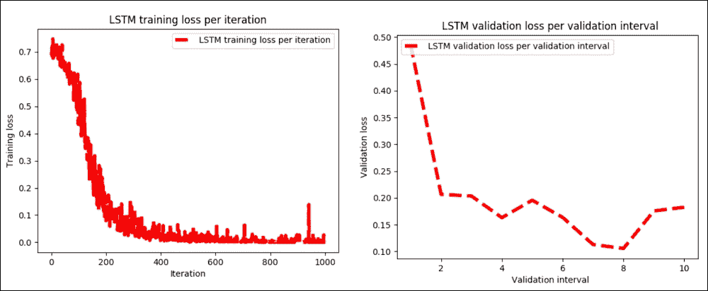圖 21：a）測試集上每次迭代的 LSTM 訓練損失，b）每個驗證間隔的 LSTM 驗證損失 如果我們檢查前面的繪圖，很明顯訓練階段和驗證階段的訓練都很順利，只有 1000 步。然而，讀者應加大訓練步驟，調整超參數，看看它是如何去。 ## 通過 TensorBoard 的可視化 現在讓我們觀察 TensorBoard 上的 TensorFlow 計算圖。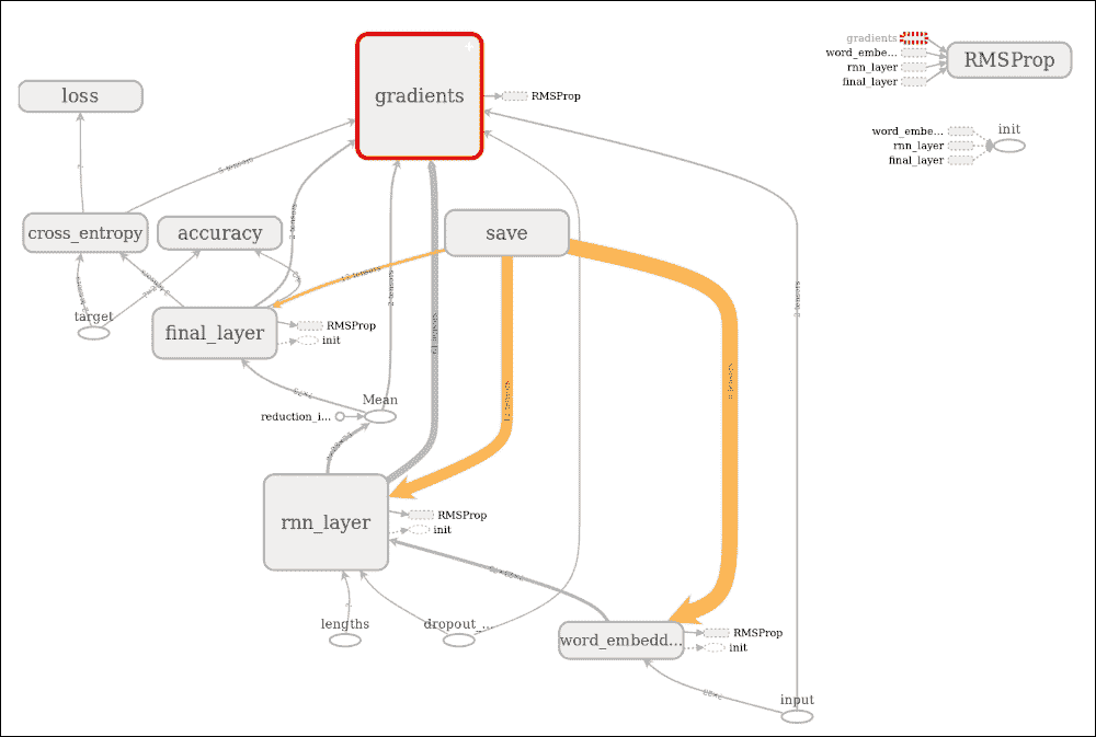只需執行以下命令并在`localhost:6006/`訪問 TensorBoard： ```py tensorboard --logdir /home/logs/ ``` 圖選項卡顯示執行圖，包括使用的梯度，`loss_op`，精度，最終層，使用的優化器（在我們的例子中是`RMSPro`），LSTM 層（即 RNN 層），嵌入層和`save_op`：  圖 22：TensorBoard 上的執行圖 執行圖顯示，我們為這種基于 LSTM 的分類器進行的情感分析計算是非常透明的。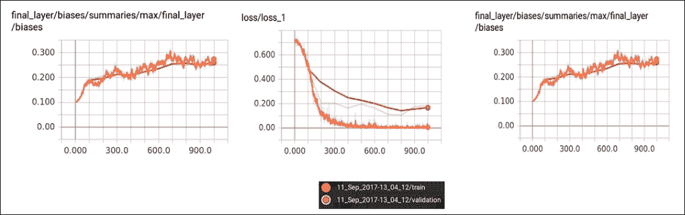我們還可以觀察層中的驗證，訓練損失，準確率和操作：  圖 23：TensorBoard 層中的驗證，訓練損失，準確率和操作 ## LSTM 模型評估 我們已經訓練了并保存了我們的 LSTM 模型。我們可以輕松恢復訓練模型并進行一些評估。我們需要準備測試集并使用先前訓練的 TensorFlow 模型對其進行預測。我們馬上做吧。首先，我們加載所需的模型： ```py import tensorflow as tf from data_preparation import Preprocessing import pickle Then we load to show the checkpoint directory where the model was saved. For our case, it was checkpoints/1505148083. ``` ### 注意 對于此步驟，使用以下命令執行`predict.py`腳本： ```py $ python3 predict.py --checkpoints_dir checkpoints/1517781236 ``` ```py # Change this path based on output by 'python3 train.py' checkpoints_dir = 'checkpoints/1517781236' ifcheckpoints_dir is None: raise ValueError('Please, a valid checkpoints directory is required (--checkpoints_dir <file name>)') ``` 現在加載測試數據集并準備它以評估模型： ```py data_lstm = Preprocessing(data_dir=data_dir, stopwords_file=stopwords_file, sequence_len=sequence_len, n_samples=n_samples, test_size=test_size, val_samples=batch_size, random_state=random_state, ensure_preprocessed=True) ``` 在上面的代碼中，完全按照我們在訓練步驟中的操作使用以下參數： ```py data_dir = 'data/' # Data directory containing 'data.csv' stopwords_file = 'data/stopwords.txt' # Path to stopwords file. sequence_len = None # Maximum sequence length n_samples= None # Set n_samples=None to use the whole dataset test_size = 0.2 batch_size = 100 #Batch size random_state = 0 # Random state used for data splitting. Default is 0 ``` 此評估方法的工作流程如下： 1. 首先，導入元圖并使用測試數據評估模型 2. 為計算創建 TensorFlow 會話 3. 導入圖并恢復其權重 4. 恢復輸入/輸出張量 5. 執行預測 6. 最后，我們在簡單的測試集上打印精度和結果 步驟 1 之前已經完成 。此代碼執行步驟 2 到 5： ```py original_text, x_test, y_test, test_seq_len = data_lstm.get_test_data(original_text=True) graph = tf.Graph() with graph.as_default(): sess = tf.Session() print('Restoring graph ...') saver = tf.train.import_meta_graph("{}/model.ckpt.meta".format(FLAGS.checkpoints_dir)) saver.restore(sess, ("{}/model.ckpt".format(checkpoints_dir))) input = graph.get_operation_by_name('input').outputs[0] target = graph.get_operation_by_name('target').outputs[0] seq_len = graph.get_operation_by_name('lengths').outputs[0] dropout_keep_prob = graph.get_operation_by_name('dropout_keep_prob').outputs[0] predict = graph.get_operation_by_name('final_layer/softmax/predictions').outputs[0] accuracy = graph.get_operation_by_name('accuracy/accuracy').outputs[0] pred, acc = sess.run([predict, accuracy], feed_dict={input: x_test, target: y_test, seq_len: test_seq_len, dropout_keep_prob: 1}) print("Evaluation done.") ``` 以下是上述代碼的輸出： ```py >>> Restoring graph ... The evaluation was done. ``` 做得好！訓練結束了，讓我們打印結果： ```py print('\nAccuracy: {0:.4f}\n'.format(acc)) for i in range(100): print('Sample: {0}'.format(original_text[i])) print('Predicted sentiment: [{0:.4f}, {1:.4f}]'.format(pred[i, 0], pred[i, 1])) print('Real sentiment: {0}\n'.format(y_test[i])) ``` 以下是上述代碼的輸出： ```py >>> Accuracy: 0.9858 Sample: I loved the Da Vinci code, but it raises many theological questions most of which are very absurd... Predicted sentiment: [0.0000, 1.0000] Real sentiment: [0\. 1.] … Sample: I'm sorry I hate to read Harry Potter, but I love the movies! Predicted sentiment: [1.0000, 0.0000] Real sentiment: [1\. 0.] … Sample: I LOVE Brokeback Mountain... Predicted sentiment: [0.0002, 0.9998] Real sentiment: [0\. 1.] … Sample: We also went to see Brokeback Mountain which totally SUCKED!!! Predicted sentiment: [1.0000, 0.0000] Real sentiment: [1\. 0.] ``` 精度高于 98%。這太棒了！但是，您可以嘗試使用調整的超參數迭代訓練以獲得更高的迭代次數，您可能會獲得更高的準確率。我把它留給讀者。 在下一節中，我們將看到如何使用 LSTM 開發更高級的 ML 項目，這被稱為使用智能手機數據集的人類活動識別。簡而言之，我們的 ML 模型將能夠將人類運動分為六類：走路，走樓上，走樓下，坐，站立和鋪設。 # LSTM 模型和人類活動識別 人類活動識別（HAR）數據庫是通過對攜帶帶有嵌入式慣性傳感器的腰部智能手機的 30 名參加日常生活活動（ADL）的參與者進行測量而建立的。目標是將他們的活動分類為前面提到的六個類別之一。 ## 數據集描述 實驗在一組 30 名志愿者中進行，年齡范圍為 19-48 歲。每個人都在腰上戴著三星 Galaxy S II 智能手機，完成了六項活動（步行，走樓上，走樓下，坐著，站著，躺著）。使用加速度計和陀螺儀，作者以 50 Hz 的恒定速率捕獲了 3 軸線性加速度和 3 軸角速度。 僅使用兩個傳感器，加速度計和陀螺儀。通過應用噪聲濾波器對傳感器信號進行預處理，然后在 2.56 秒的固定寬度滑動窗口中采樣，重疊 50%。這樣每個窗口提供 128 個讀數。來自傳感器加速度信號的重力和身體運動分量通過巴特沃斯低通濾波器分離成身體加速度和重力。 欲了解更多信息，請參閱本文：Davide Anguita，Alessandro Ghio，Luca Oneto，Xavier Parra 和 Jorge L. Reyes-Ortiz，使用智能手機進行人類活動識別的公共領域數據集和第 21 屆關于人工神經網絡的歐洲研討會，計算智能和機器學習，ESANN 2013.比利時布魯日 24-26，2013 年 4 月。 為簡單起見，假設重力僅具有少量低頻分量。因此，使用 0.3Hz 截止頻率的濾波器。從每個窗口，通過計算來自時域和頻域的變量找到特征向量。 已經對實驗進行了視頻記錄以便于手動標記數據。數據集已被隨機分為兩組，其中 70% 的志愿者被選中用于訓練數據，30% 用于測試數據。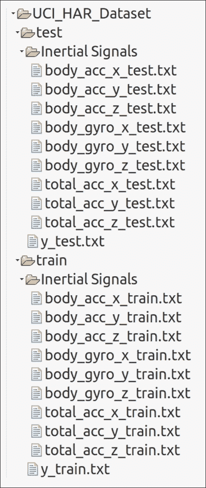當我瀏覽數據集時，訓練集和測試集都具有以下文件結構：  圖 24：HAR 數據集文件結構 對于數據集中的每條記錄，提供以下內容： * 來自加速度計的三軸加速度和估計的車身加速度 * 來自陀螺儀傳感器的三軸角速度 * 具有時域和頻域變量的 561 特征向量 * 它的活動標簽 * 進行實驗的受試者的標識符 因此，我們知道需要解決的問題。現在是探索技術和相關挑戰的時候了。 ## 用于 HAR 的 LSTM 模型的工作流程 整個算法有以下工作流程： 1. 加載數據。 2. 定義超參數。 3. 使用命令式編程和超參數設置 LSTM 模型。 4. 應用批量訓練。也就是說，選擇一批數據，將其提供給模型，然后在一些迭代之后，評估模型并打印批次損失和準確率。 5. 輸出圖的訓練和測試誤差。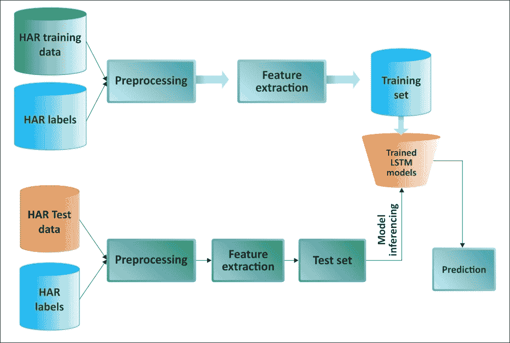 可以遵循上述步驟并構建一個管道：  圖 25：用于 HAR 的基于 LSTM 的管道 ## 為 HAR 實現 LSTM 模型 首先，我們導入所需的包和模塊： ```py import numpy as np import matplotlib import matplotlib.pyplot as plt import tensorflow as tf from sklearn import metrics from tensorflow.python.framework import ops import warnings import random warnings.filterwarnings("ignore") os.environ['TF_CPP_MIN_LOG_LEVEL'] = '3' ``` 如前所述，`INPUT_SIGNAL_TYPES`包含一些有用的常量。它們是神經網絡的單獨標準化輸入特征： ```py INPUT_SIGNAL_TYPES = [ "body_acc_x_", "body_acc_y_", "body_acc_z_", "body_gyro_x_", "body_gyro_y_", "body_gyro_z_", "total_acc_x_", "total_acc_y_", "total_acc_z_" ] ``` 標簽在另一個數組中定義 - 這是用于學習如何分類的輸出類： ```py LABELS = [ "WALKING", "WALKING_UPSTAIRS", "WALKING_DOWNSTAIRS", "SITTING", "STANDING", "LAYING" ] ``` 我們現在假設您已經從[此鏈接](https://archive.ics.uci.edu/ml/machine-learning-databases/00240/UCI HAR Dataset.zip)下載了 HAR 數據集并輸入了名為`UCIHARDataset`的文件夾（或者您可以選擇聽起來更合適的合適名稱）。此外，我們需要提供訓練和測試集的路徑： ```py DATASET_PATH = "UCIHARDataset/" print("\n" + "Dataset is now located at: " + DATASET_PATH) TRAIN = "train/" TEST = "test/" ``` 然后我們加載并根據由`[Array [Array [Float]]]`格式的`INPUT_SIGNAL_TYPES`數組定義的輸入信號類型，映射每個`.txt`文件的數據。`X`表示神經網絡的訓練和測試輸入： ```py def load_X(X_signals_paths): X_signals = [] for signal_type_path in X_signals_paths: file = open(signal_type_path, 'r') # Read dataset from disk, dealing with text files' syntax X_signals.append( [np.array(serie, dtype=np.float32) for serie in [ row.replace(' ', ' ').strip().split(' ') for row in file ]] ) file.close() return np.transpose(np.array(X_signals), (1, 2, 0)) X_train_signals_paths = [DATASET_PATH + TRAIN + "Inertial Signals/" + signal + "train.txt" for signal in INPUT_SIGNAL_TYPES] X_test_signals_paths = [DATASET_PATH + TEST + "Inertial Signals/" + signal + "test.txt" for signal in INPUT_SIGNAL_TYPES] X_train = load_X(X_train_signals_paths) X_test = load_X(X_test_signals_paths) ``` 然后我們加載`y`，神經網絡的訓練和測試輸出的標簽： ```py def load_y(y_path): file = open(y_path, 'r') # Read dataset from disk, dealing with text file's syntax y_ = np.array( [elem for elem in [ row.replace(' ', ' ').strip().split(' ') for row in file ]], dtype=np.int32 ) file.close() # We subtract 1 to each output class for 0-based indexing return y_ - 1 y_train_path = DATASET_PATH + TRAIN + "y_train.txt" y_test_path = DATASET_PATH + TEST + "y_test.txt" y_train = load_y(y_train_path) y_test = load_y(y_test_path) ``` 讓我們看看一些數據集的統計數據，例如訓練系列的數量（如前所述，每個系列之間有 50% 的重疊），測試系列的數量，每個系列的時間步數，以及每個時間步輸入參數： ```py training_data_count = len(X_train) test_data_count = len(X_test) n_steps = len(X_train[0]) n_input = len(X_train[0][0]) print("Number of training series: "+ trainingDataCount) print("Number of test series: "+ testDataCount) print("Number of timestep per series: "+ nSteps) print("Number of input parameters per timestep: "+ nInput) ``` 以下是上述代碼的輸出： ```py >>> Number of training series: 7352 Number of test series: 2947 Number of timestep per series: 128 Number of input parameters per timestep: 9 ``` 現在讓我們為訓練定義一些核心參數定義。整個神經網絡的結構可以通過枚舉這些參數和使用 LSTM 這一事實來概括： ```py n_hidden = 32 # Hidden layer num of features n_classes = 6 # Total classes (should go up, or should go down) learning_rate = 0.0025 lambda_loss_amount = 0.0015 training_iters = training_data_count * 300 #Iterate 300 times batch_size = 1500 display_iter = 30000 # to show test set accuracy during training ``` 我們已經定義了所有核心參數和網絡參數。這些是隨機選擇。我沒有進行超參數調整，但仍然運行良好。因此，我建議使用網格搜索技術調整這些超參數。有許多在線資料可供使用。 然而，在構建 LSTM 網絡并開始訓練之前，讓我們打印一些調試信息，以確保執行不會中途停止： ```py print("Some useful info to get an insight on dataset's shape and normalization:") print("(X shape, y shape, every X's mean, every X's standard deviation)") print(X_test.shape, y_test.shape, np.mean(X_test), np.std(X_test)) print("The dataset is therefore properly normalized, as expected, but not yet one-hot encoded.") ``` 以下是上述代碼的輸出： ```py >>> Some useful info to get an insight on dataset's shape and normalization: (X shape, y shape, every X's mean, every X's standard deviation) (2947, 128, 9) (2947, 1) 0.0991399 0.395671 ``` 數據集是 ，因此按預期正確標準化，但尚未進行單熱編碼。 現在訓練數據集處于校正和標準化順序，現在是構建 LSTM 網絡的時候了。以下函數從給定參數返回 TensorFlow LSTM 網絡。此外，兩個 LSTM 單元堆疊在一起，這增加了神經網絡的深度： ```py def LSTM_RNN(_X, _weights, _biases): _X = tf.transpose(_X, [1,0,2])# permute n_steps & batch_size _X = tf.reshape(_X, [-1, n_input]) _X = tf.nn.relu(tf.matmul(_X, _weights['hidden']) + _biases['hidden']) _X = tf.split(_X, n_steps, 0) lstm_cell_1 = tf.nn.rnn_cell.BasicLSTMCell(n_hidden, forget_bias=1.0, state_is_tuple=True) lstm_cell_2 = tf.nn.rnn_cell.BasicLSTMCell(n_hidden, forget_bias=1.0, state_is_tuple=True) lstm_cells = tf.nn.rnn_cell.MultiRNNCell([lstm_cell_1, lstm_cell_2], state_is_tuple=True) outputs, states = tf.contrib.rnn.static_rnn(lstm_cells, _X, dtype=tf.float32) lstm_last_output = outputs[-1] return tf.matmul(lstm_last_output, _weights['out']) + _biases['out'] ``` 如果我們仔細查看前面的代碼片段，我們可以看到我們得到了“多對一”樣式分類器的最后一步輸出特征。現在，問題是什么是多對一 RNN 分類器？好吧，類似于圖 5，我們接受特征向量的時間序列（每個時間步長一個向量）并將它們轉換為輸出中的概率向量以進行分類。 現在我們已經能夠構建我們的 LSTM 網絡，我們需要將訓練數據集準備成批量。以下函數從`(X|y)_train`數據中獲取`batch_size`數據量： ```py def extract_batch_size(_train, step, batch_size): shape = list(_train.shape) shape[0] = batch_size batch_s = np.empty(shape) for i in range(batch_size): index = ((step-1)*batch_size + i) % len(_train) batch_s[i] = _train[index] return batch_s ``` 之后，我們需要將數字索引的輸出標簽編碼為二元類別。然后我們用`batch_size`執行訓練步驟。例如，`[[5], [0], [3]]`需要轉換為類似于`[[0, 0, 0, 0, 0, 1], [1, 0, 0, 0, 0, 0], [0, 0, 0, 1, 0, 0]]`的形狀。好吧，我們可以用單熱編碼來做到這一點。以下方法執行完全相同的轉換： ```py def one_hot(y_): y_ = y_.reshape(len(y_)) n_values = int(np.max(y_)) + 1 return np.eye(n_values)[np.array(y_, dtype=np.int32)] ``` 優秀的！我們的數據集準備就緒，因此我們可以開始構建網絡。首先，我們為輸入和標簽創建兩個單獨的占位符： ```py x = tf.placeholder(tf.float32, [None, n_steps, n_input]) y = tf.placeholder(tf.float32, [None, n_classes]) ``` 然后我們創建所需的權重向量： ```py weights = { 'hidden': tf.Variable(tf.random_normal([n_input, n_hidden])), 'out': tf.Variable(tf.random_normal([n_hidden, n_classes], mean=1.0)) } ``` 然后我們創建所需的偏向量： ```py biases = { 'hidden': tf.Variable(tf.random_normal([n_hidden])), 'out': tf.Variable(tf.random_normal([n_classes])) } ``` 然后我們通過傳遞輸入張量，權重向量和偏置向量來構建模型，如下所示： ```py pred = LSTM_RNN(x, weights, biases) ``` 此外，我們還需要計算`cost`操作，正則化，優化器和評估。我們使用 L2 損失進行正則化，這可以防止這種過度殺傷神經網絡過度適應訓練中的問題： ```py l2 = lambda_loss_amount * sum(tf.nn.l2_loss(tf_var) for tf_var in tf.trainable_variables()) cost = tf.reduce_mean(tf.nn.softmax_cross_entropy_with_logits_v2(labels=y, logits=pred)) + l2 optimizer = tf.train.AdamOptimizer(learning_rate=learning_rate).minimize(cost) correct_pred = tf.equal(tf.argmax(pred,1), tf.argmax(y,1)) accuracy = tf.reduce_mean(tf.cast(correct_pred, tf.float32)) Great! So far, everything has been fine. Now we are ready to train the neural network. First, we create some lists to hold some training's performance: ``` ```py test_losses = [] test_accuracies = [] train_losses = [] train_accuracies = [] ``` 然后我們創建一個 TensorFlow 會話，啟動圖并初始化全局變量： ```py sess = tf.InteractiveSession(config=tf.ConfigProto(log_device_placement=False)) init = tf.global_variables_initializer() sess.run(init) ``` 然后我們在每個循環中以`batch_size`數量的示例數據執行訓練步驟。我們首先使用批量數據進行訓練，然后我們僅在幾個步驟評估網絡以加快訓練速度。另外，我們評估測試集（這里沒有學習，只是診斷評估）。最后，我們打印結果： ```py step = 1 while step * batch_size <= training_iters: batch_xs = extract_batch_size(X_train, step, batch_size) batch_ys = one_hot(extract_batch_size(y_train, step, batch_size)) _, loss, acc = sess.run( [optimizer, cost, accuracy], feed_dict={ x: batch_xs, y: batch_ys } ) train_losses.append(loss) train_accuracies.append(acc) if (step*batch_size % display_iter == 0) or (step == 1) or (step * batch_size > training_iters): print("Training iter #" + str(step*batch_size) + \": Batch Loss = " + "{:.6f}".format(loss) + \", Accuracy = {}".format(acc)) loss, acc = sess.run( [cost, accuracy], feed_dict={ x: X_test, y: one_hot(y_test) } ) test_losses.append(loss) test_accuracies.append(acc) print("PERFORMANCE ON TEST SET: " + \ "Batch Loss = {}".format(loss) + \ ", Accuracy = {}".format(acc)) step += 1 print("Optimization Finished!") one_hot_predictions, accuracy, final_loss = sess.run( [pred, accuracy, cost], feed_dict={ x: X_test, y: one_hot(y_test) }) test_losses.append(final_loss) test_accuracies.append(accuracy) print("FINAL RESULT: " + \ "Batch Loss = {}".format(final_loss) + \ ", Accuracy = {}".format(accuracy)) ``` 以下是上述代碼的輸出： ```py >>> Training iter #1500: Batch Loss = 3.266330, Accuracy = 0.15733332931995392 PERFORMANCE ON TEST SET: Batch Loss = 2.6498606204986572, Accuracy = 0.15473362803459167 Training iter #30000: Batch Loss = 1.538126, Accuracy = 0.6380000114440918 …PERFORMANCE ON TEST SET: Batch Loss = 0.5507552623748779, Accuracy = 0.8924329876899719 Optimization Finished! FINAL RESULT: Batch Loss = 0.6077192425727844, Accuracy = 0.8686800003051758 ``` 做得好！ 訓練進展順利。但是，視覺概述會更有用： ```py indep_train_axis = np.array(range(batch_size, (len(train_losses)+1)*batch_size, batch_size)) plt.plot(indep_train_axis, np.array(train_losses), "b--", label="Train losses") plt.plot(indep_train_axis, np.array(train_accuracies), "g--", label="Train accuracies") indep_test_axis = np.append(np.array(range(batch_size, len(test_losses)*display_iter, display_iter)[:-1]), [training_iters]) plt.plot(indep_test_axis, np.array(test_losses), "b-", label="Test losses") plt.plot(indep_test_axis, np.array(test_accuracies), "g-", label="Test accuracies") plt.title("Training session's progress over iterations") plt.legend(loc='upper right', shadow=True) plt.ylabel('Training Progress (Loss or Accuracy values)') plt.xlabel('Training iteration') plt.show() ``` 以下是上述代碼的輸出： ```py >>> ```  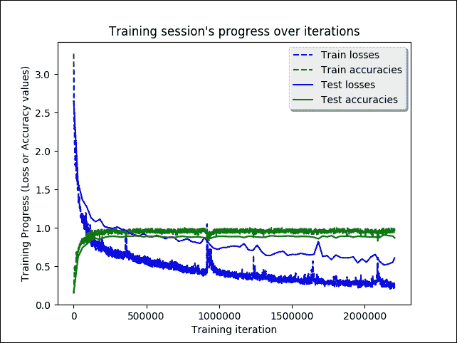圖 26：迭代時的 LSTM 訓練過程 我們需要計算其他表現指標，例如`accuracy`，`precision`，`recall`和`f1`度量： ```py predictions = one_hot_predictions.argmax(1) print("Testing Accuracy: {}%".format(100*accuracy)) print("") print("Precision: {}%".format(100*metrics.precision_score(y_test, predictions, average="weighted"))) print("Recall: {}%".format(100*metrics.recall_score(y_test, predictions, average="weighted"))) print("f1_score: {}%".format(100*metrics.f1_score(y_test, predictions, average="weighted"))) ``` 以下是上述代碼的輸出： ```py >>> Testing Accuracy: 89.51476216316223% Precision: 89.65053428376297% Recall: 89.51476077366813% f1_score: 89.48593061935716% ``` 由于我們正在接近的問題是多類分類，因此繪制混淆矩陣是有意義的： ```py print("") print ("Showing Confusion Matrix") cm = metrics.confusion_matrix(y_test, predictions) df_cm = pd.DataFrame(cm, LABELS, LABELS) plt.figure(figsize = (16,8)) plt.ylabel('True label') plt.xlabel('Predicted label') sn.heatmap(df_cm, annot=True, annot_kws={"size": 14}, fmt='g', linewidths=.5) plt.show() ``` 以下是上述代碼的輸出： ```py >>> ```  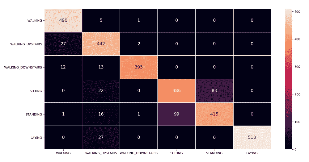圖 27：多類混淆矩陣（預測與實際） 在混淆矩陣中，訓練和測試數據不是在類之間平均分配，因此正常情況下，超過六分之一的數據在最后一類中被正確分類。話雖如此，我們已經設法達到約 87% 的預測準確率。我們很快就會看到更多分析。它可能更高，但是訓練是在 CPU 上進行的，因此它的精度很低，當然需要很長時間。因此，我建議你在 GPU 上訓練，以獲得更好的結果。此外，調整超參數可能是一個不錯的選擇。 # 總結 LSTM 網絡配備了特殊的隱藏單元，稱為存儲單元，其目的是長時間記住先前的輸入。這些單元在每個時刻采用先前狀態和網絡的當前輸入作為輸入。通過將它們與內存的當前內容相結合，并通過其他單元的門控機制決定保留什么以及從內存中刪除什么，LSTM 已被證明是非常有用的并且是學習長期依賴性的有效方式。 在本章中，我們討論了 RNN。我們看到了如何使用具有高時間依賴性的數據進行預測。我們看到了如何開發幾種真實的預測模型，使用 RNN 和不同的架構變體使預測分析更容易。我們從 RNN 的理論背景開始。 然后我們看了幾個例子，展示了一種實現圖像分類預測模型，電影和產品情感分析以及 NLP 垃圾郵件預測的系統方法。然后我們看到了如何開發時間序列數據的預測模型。最后，我們看到了 RNN 用于人類活動識別的更高級應用，我們觀察到分類準確率約為 87%。 DNN 以統一的方式構造，使得在網絡的每一層，數千個相同的人工神經元執行相同的計算。因此，DNN 的架構非常適合 GPU 可以有效執行的計算類型。 GPU 具有優于 CPU 的額外優勢；這些包括具有更多計算單元并具有更高的帶寬用于存儲器檢索。 此外，在許多需要大量計算工作的深度學習應用中，可以利用 GPU 的圖形特定功能來進一步加速計算。在下一章中，我們將看到如何使訓練更快，更準確，甚至在節點之間分配。