# 八、TensorFlow 2 和循環神經網絡 包括卷積網絡（CNN）在內的許多神經網絡體系結構的主要缺點之一是它們不允許處理順序數據。 換句話說，一個完整的特征（例如圖像）必須一次全部呈現。 因此，輸入是固定長度張量，而輸出必須是固定長度張量。 先前特征的輸出值也不會以任何方式影響當前特征。 同樣，所有輸入值（和輸出值）都應視為彼此獨立。 例如，在我們的`fashion_mnist`模型（第 4 章“使用 TensorFlow 2的監督機器學習”）中，每個輸入時尚圖像都獨立于并且完全不了解先前圖像。 **循環神經網絡**（**RNN**）克服了這個問題，并使許多新的應用成為可能。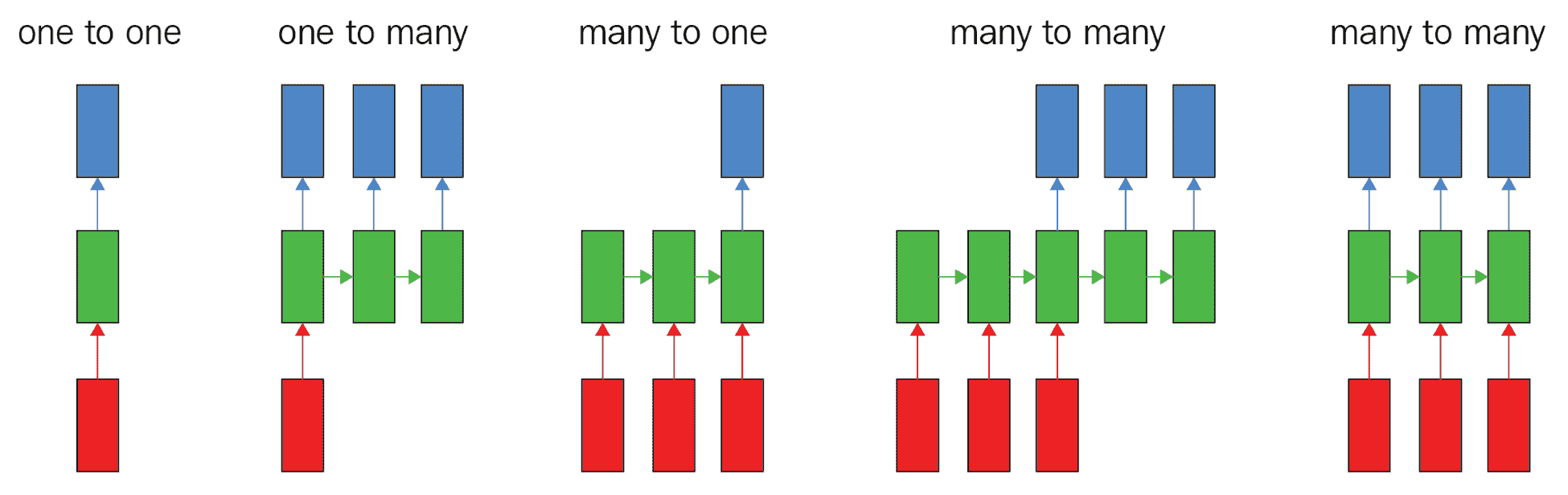 在本章中，我們將研究以下主題： * 神經網絡處理模式 * 循環架構 * RNN 的應用 * 我們的 RNN 示例的代碼 * 建立并實例化我們的模型 * 訓練和使用我們的模型 # 神經網絡處理模式 下圖說明了各種神經網絡處理模式：  矩形代表張量，箭頭代表函數，紅色是輸入，藍色是輸出，綠色是張量狀態。 從左到右，我們有以下內容： * 普通前饋網絡，固定尺寸的輸入和固定尺寸的輸出，例如圖像分類 * 序列輸出，例如，拍攝一張圖像并輸出一組用于標識圖像中項目的單詞的圖像字幕 * 序列輸入，例如情感識別（如我們的 IMDb 應用），其中句子被分為正面情感或負面情感 * 序列輸入和輸出，例如機器翻譯，其中 RNN 接受英語句子并將其翻譯為法語輸出 * 逐幀同步輸入和輸出的序列，例如，類似于視頻分類的兩者 # 循環架構 因此，需要一種新的體系結構來處理順序到達的數據，并且其輸入值和輸出值中的一個或兩個具有可變長度，例如，語言翻譯應用中句子中的單詞。 在這種情況下，模型的輸入和輸出都具有不同的長度，就像之前的第四種模式一樣。 同樣，為了預測給定當前詞的后續詞，還需要知道先前的詞。 這種新的神經網絡架構稱為 RNN，專門設計用于處理順序數據。 出現術語**循環**是因為此類模型對序列的每個元素執行相同的計算，其中每個輸出都依賴于先前的輸出。 從理論上講，每個輸出都取決于所有先前的輸出項，但實際上，RNN 僅限于回顧少量步驟。 這種布置等效于具有存儲器的 RNN，該存儲器可以利用先前的計算結果。 RNN 用于順序輸入值，例如時間序列，音頻，視頻，語音，文本，財務和天氣數據。 它們在消費產品中的使用示例包括 Apple 的 Siri，Google 翻譯和亞馬遜的 Alexa。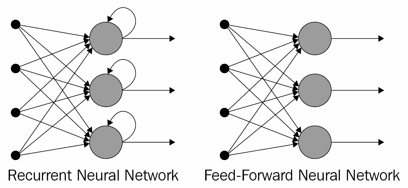 將傳統前饋網絡與 RNN 進行比較的示意圖如下：  每個 RNN 單元上的回送代表*記憶*。 前饋網絡無法區分序列中的項目順序，而 RNN 從根本上取決于項目的順序。 例如，假設前饋網絡接收到輸入字符串`aardvark`：到輸入為`d`時，網絡已經忘記了先前的輸入值為`a`，`a`和`r`，因此無法預測下一個`va`。 另一方面，在給定相同輸入的情況下，循環網絡“記住”先前的輸入值為`a`，`a`和`r`，因此*有可能*根據其先前的訓練來預測`va`是下一個。 RNN 的每個單獨項目到網絡的輸入稱為**時間步長**。 因此，例如，在字符級 RNN 中，每個字符的輸入都是一個時間步。 下圖說明了 RNN 的*展開*。 時間步長從`t = 0`開始，輸入為`X[0]`，一直到時間步長`t = t`，輸入為`X[t]`，相應的輸出值為`h[0]`至`h[t]`，如下圖所示：  展開式循環神經網絡 RNN 在稱為**沿時間反向傳播**（**BPTT**）的過程中通過反向傳播進行訓練。 在此可以想象 RNN 的展開（也稱為**展開**）會創建一系列神經網絡，并且會針對每個時間步長計算誤差并將其合并，以便可以使用反向傳播更新網絡中的權重。 例如，為了計算梯度，從而計算誤差，在時間步`t = 6`時，我們將向后傳播五個步，并對梯度求和。 但是，在嘗試學習長期依賴關系時（即在相距很遠的時間步之間），這種方法存在問題，因為梯度可能變得太小而使學習變得不可能或非常緩慢，或者它們可能變得太大并淹沒了網絡。 這被稱為消失/爆炸梯度問題，并且已經發明了各種修改方法來解決它，包括**長短期記憶**（**LSTM**）網絡和**門控循環單元**（**GRU** **s**），我們將在以后使用。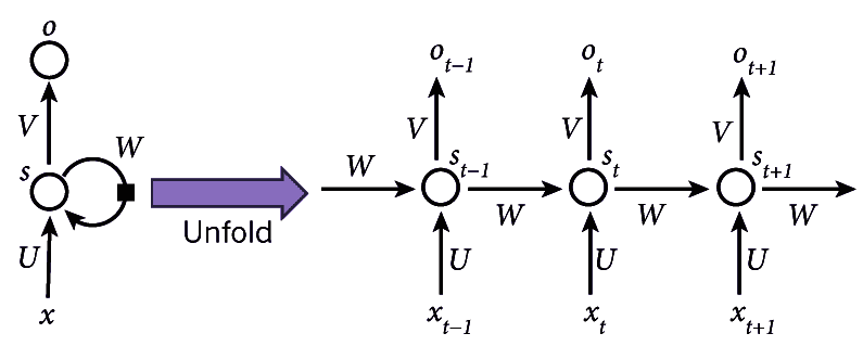 下圖顯示了有關展開（或展開）的更多詳細信息：  循環神經網絡的示意圖 在該圖中，我們可以看到以下內容： * `x[t]`是時間步長`t`的輸入。 例如，`x[t]`可以是基于字符的 RNN 中的第十個字符，表示為來自字符集的索引。 * `s[t]`是時間步`t`的隱藏狀態，因此是網絡的內存。 * `s[t]`的計算公式為`s[t] = f(Ux[t] + Ws[t-1])`，其中`f`是非線性函數，例如 ReLU。 `U`，`V`和`W`是權重。 * `o[t]`是時間步長`t`的輸出。 例如，如果我們要計算字符序列中的下一個字母，它將是字符集`o[t] = Vs[t]`的概率向量。 如前所述，我們可以將`s[t]`視為網絡的內存，因為它包含有關網絡中較早時間步長發生了什么的信息。 請注意，權重`U`，`V`和`W`在每個步驟中都是共享的，因為我們在每個步驟都執行相同的計算，只是使用不同的輸入值（ 結果是學習權重的數量大大減少了）。 還要注意，我們可能不需要每個時間步長的輸出值（如圖所示）。 如果我們要進行情感分析，每個步驟都是一個詞，比如說電影評論，那么我們可能只關心最終的輸出（正面或負面）。 現在，讓我們看一個使用 RNN 的有趣示例，在該示例中，我們嘗試以給定的寫作風格創建文本。 # RNN 的應用 在此應用中，我們將看到如何使用基于字符的循環神經網絡創建文本。 更改要使用的文本的語料庫很容易（請參見下面的示例）； 在這里，我們將使用查爾斯·狄更斯（Charles Dickens）的小說《偉大的期望》。 我們將在此文本上訓練網絡，以便如果我們給它一個字符序列，例如`thousan`，它將產生序列中的下一個字符`d`。 此過程可以繼續進行，可以通過在不斷演變的序列上反復調用模型來創建更長的文本序列。 這是訓練模型之前創建的文本的示例： ```py Input: 'o else is there to inform?”\n\n“Is there no chance person who might identify you in the street?” said\n' Next Char Predictions: "dUFdZ!mig())'(ZIon“4g&HZ”@\nWGWtlinnqQY*dGJ7ioU'6(vLKL&cJ29LG'lQW8n-,M!JSVy”cjN;1cH\ndEEeMXhtW$U8Mt&sp" ``` 這是一些文本，其中包含`Pip`序列，該序列是在模型經過 0.1 個溫度（請參閱下文）進行 100 個周期（約 10 秒每個）的訓練后創建的： ```py Pip; it was not to be done. I had been a little while I was a look out and the strength of considerable particular by the windows of the rest of his prospering look at the windows of the room wing and the courtyard in the morning was the first time I had been a very much being strictly under the wall of my own person to me that he had done my sister, and I went on with the street common, I should have been a very little for an air of the river by the fire. For the man who was all the time of the money. My dear Herbert, who was a little way to the marshes he had ever seemed to have had once more than once and the more was a ragged hand before I had ever seemed to have him a dreadful loveriement in his head and with a falling to the table, and I went on with his arms, I saw him ever so many times, and we all the courtyard to the fire to be so often to be on some time when I saw his shoulder as if it were a long time in the morning I was a woman and a singer at the tide was remained by the ``` 對于不了解語法或拼寫的系統來說，這并不是一個壞結果。 這顯然是荒謬的，但那時我們并不是在追求理性。 只有一個不存在的單詞（`loveriement`）。 因此，網絡已經完成了學習拼寫和學習單詞是文本單元的工作。 還要注意，在下面的代碼中，僅在短序列（`sequence_length = 100`）上訓練網絡。 接下來，我們將查看用于設置，訓練和測試循環神經網絡的代碼。 # 我們的 RNN 示例的代碼 此應用基于 Google 根據 Apache 2 許可提供的應用。 像往常一樣，我們會將代碼分解成片段，然后將您引到存儲庫中獲取許可證和完整的工作版本。 首先，我們有模塊導入，如下所示： ```py import tensorflow as tf import numpy as np import os import time ``` 接下來，我們有文本文件的下載鏈接。 您可以通過在`file`中指定文件名和在`url`中指定文件的完整 URL，輕松地將其更改為所需的任何文本： ```py file='1400-0.txt' url='https://www.gutenberg.org/files/1400/1400-0.txt' # Great Expectations by Charles Dickens ``` 然后，我們為該文件設置了 Keras `get_file()`工具，如下所示： ```py path = tf.keras.utils.get_file(file,url) ``` 然后，我們打開并讀取文件，并以字符為單位查看文件的長度： ```py text = open(path).read() print ('Length of text: {} characters'.format(len(text))) ``` 在文件開頭沒有我們不需要的文本，因此我們將其剝離掉，然后再看一下前幾個字符就很有幫助了，接下來我們要做： ```py # strip off text we don't need text = text[835:] # Take a look at the first 300 characters in text print(text[:300]) ``` 輸出應如下所示： ```py My father's family name being Pirrip, and my Christian name Philip, my infant tongue could make of both names nothing longer or more explicit than Pip. So, I called myself Pip, and came to be called Pip. I give Pirrip as my father's family name, on the authority of his tombstone and my sister,--Mrs ``` 現在，讓我們看一下文本中有多少個唯一字符，使用一組字符來獲取它們，并按其 ASCII 碼的順序對其進行排序： ```py # The unique characters in the file vocabulary = sorted(set(text)) print ('{} unique characters.'.format(len(vocabulary))) ``` 這應該提供 84 個唯一字符。 接下來，我們創建一個字典，其中字符是鍵，而連續的整數是值。 這樣我們就可以找到索引，表示任何給定字符的數值： ```py # Create a dictionary of unique character keys to index values char_to_index = {char:index for index, char in enumerate(vocabulary)} print(char_to_index) ``` 輸出如下： ```py {'\n': 0, ' ': 1, '!': 2, '$': 3, '%': 4, '&': 5, "'": 6, '(': 7, ')': 8, '*': 9, ',': 10, '-': 11, '.': 12, '/': 13, '0': 14, '1': 15, '2': 16, '3': 17, '4': 18, '5': 19, '6': 20, '7': 21, '8': 22, '9': 23, ':': 24, ';': 25, '?': 26, '@': 27, 'A': 28, 'B': 29, 'C': 30, 'D': 31, 'E': 32, 'F': 33, 'G': 34, 'H': 35, 'I': 36, 'J': 37, 'K': 38, 'L': 39, 'M': 40, 'N': 41, 'O': 42, 'P': 43, 'Q': 44, 'R': 45, 'S': 46, 'T': 47, 'U': 48, 'V': 49, 'W': 50, 'X': 51, 'Y': 52, 'Z': 53, 'a': 54, 'b': 55, 'c': 56, 'd': 57, 'e': 58, 'f': 59, 'g': 60, 'h': 61, 'i': 62, 'j': 63, 'k': 64, 'l': 65, 'm': 66, 'n': 67, 'o': 68, 'p': 69, 'q': 70, 'r': 71, 's': 72, 't': 73, 'u': 74, 'v': 75, 'w': 76, 'x': 77, 'y': 78, 'z': 79, 'ê': 80, '?': 81, '“': 82, '”': 83} ``` 我們還需要將字符存儲在數組中。 這樣我們就可以找到與任何給定數值對應的字符，即`index`： ```py index_to_char = np.array(vocabulary) print(index_to_char) ``` 輸出如下： ```py ['\n' ' ' '!' '$' '%' '&' "'" '(' ')' '*' ',' '-' '.' '/' '0' '1' '2' '3' '4' '5' '6' '7' '8' '9' ':' ';' '?' '@' 'A' 'B' 'C' 'D' 'E' 'F' 'G' 'H' 'I' 'J' 'K' 'L' 'M' 'N' 'O' 'P' 'Q' 'R' 'S' 'T' 'U' 'V' 'W' 'X' 'Y' 'Z' 'a' 'b' 'c' 'd' 'e' 'f' 'g' 'h' 'i' 'j' 'k' 'l' 'm' 'n' 'o' 'p' 'q' 'r' 's' 't' 'u' 'v' 'w' 'x' 'y' 'z' 'ê' '?' '“' '”'] ``` 現在，我們正在使用的整個文本已轉換為我們作為字典創建的整數數組`char_to_index`： ```py text_as_int = np.array([char_to_index[char] for char in text] ``` 這是字符及其索引的示例： ```py print('{') for char,_ in zip(char_to_index, range(20)): print(' {:4s}: {:3d},'.format(repr(char), char_to_index[char])) print(' ...\n}') ``` 輸出如下： ```py { '\n': 0, ' ' : 1, '!' : 2, '$' : 3, '%' : 4, '&' : 5, "'" : 6, '(' : 7, ')' : 8, '*' : 9, ',' : 10, '-' : 11, '.' : 12, '/' : 13, '0' : 14, '1' : 15, '2' : 16, '3' : 17, '4' : 18, '5' : 19, ... } ``` 接下來，查看文本如何映射為整數很有用； 這是前幾個： ```py # Show how the first 15 characters from the text are mapped to integers print ('{} ---- characters mapped to int ---- > {}'.format(repr(text[:15]), text_as_int[:15])) ``` 輸出如下： ```py "My father's fam" ---- characters mapped to int ---- > [40 78 1 59 54 73 61 58 71 6 72 1 59 54 66] ``` 然后，我們設置每個輸入的句子長度，并因此設置訓練周期中的示例數： ```py # The maximum length sentence we want for a single input in characters sequence_length = 100 examples_per_epoch = len(text)//seq_length ``` 接下來，我們創建`data.Dataset`以在以后的訓練中使用： ```py # Create training examples / targets char_dataset = tf.data.Dataset.from_tensor_slices(text_as_int) # Display , sanity check for char in char_dataset.take(5): print(index_to_char[char.numpy()]) ``` 輸出如下： ```py M y f a ``` 我們需要批量此數據以將其饋送到我們的 RNN，因此接下來我們要這樣做： ```py sequences = char_dataset.batch(sequence_length+1, drop_remainder=True) ``` 請記住，我們已經設置了`sequence_length = 100`，所以批量中的字符數是 101。 現在，我們有了一個函數來創建我們的輸入數據和目標數據（必需的輸出）。 該函數返回我們一直在處理的文本以及相同的文本，但是一起移動了一個字符，即，如果第一個單詞是`Python`和`sequence_length = 5`，則該函數返回`Pytho`和`ython` 。 然后，我們通過連接輸入和輸出字符序列來創建數據集： ```py def split_input_target(chunk): input_text = chunk[:-1] target_text = chunk[1:] return input_text, target_text dataset = sequences.map(split_input_target) ``` 接下來，我們執行另一個健全性檢查。 我們使用先前創建的數據集來顯示輸入和目標數據。 請注意，`dataset.take(n)`方法從數據集中返回`n`批次。 在這里還請注意，由于我們已經啟用了急切執行（當然，默認情況下，在 TensorFlow 2 中是這樣），因此我們可以使用`numpy()`方法來查找張量的值： ```py for input_example, target_example in dataset.take(1): print ('Input data: ', repr(''.join(index_to_char[input_example.numpy()]))) #101 characters print ('Target data:', repr(''.join(index_to_char[target_example.numpy()]))) ``` 輸出如下： ```py Input data: "My father's family name being Pirrip, and my Christian name Philip, my\ninfant tongue could make of b" Target data: "y father's family name being Pirrip, and my Christian name Philip, my\ninfant tongue could make of bo" ``` 現在，我們可以通過幾個步驟顯示輸入和預期輸出： ```py for char, (input_index, target_index) in enumerate(zip(input_example[:5], target_example[:5])): print("Step {:4d}".format(char)) print(" input: {} ({:s})".format(input_index, repr(index_to_char[input_index]))) print(" expected output: {} ({:s})".format(target_index, repr(index_to_char[target_index]))) ``` 以下是此輸出： ```py Step 0: input: 40 ('M'), expected output: 78 ('y') Step 1: input: 78 ('y'), expected output: 1 (' ') Step 2: input: 1 (' '), expected output: 59 ('f') Step 3: input: 59 ('f'), expected output: 54 ('a') Step 4: input: 54 ('a'), expected output: 73 ('t') ``` 接下來，我們為訓練進行設置，如下所示： ```py # how many characters in a batch batch = 64 # the number of training steps taken in each epoch steps_per_epoch = examples_per_epoch//batch # note integer division # TF data maintains a buffer in memory in which to shuffle data # since it is designed to work with possibly endless data buffer = 10000 dataset = dataset.shuffle(buffer).batch(batch, drop_remainder=True) # call repeat() on dataset so data can be re-fed into the model from the beginning dataset = dataset.repeat() dataset ``` 這給出了以下數據集結構： ```py <RepeatBatchDataset shapes: ((64, 100), (64, 100)), types: (tf.int64, tf.int64)> ``` 此處，`64`是批次大小，`100`是序列長度。 以下是我們訓練所需的一些值： ```py # The vocabulary length in characters vocabulary_length = len(vocabulary) # The embedding dimension embedding_dimension = 256 # The number of recurrent neural network units recurrent_nn_units = 1024 ``` 我們正在使用 GRU，在 **CUDA 深度神經網絡**（**cuDNN**）庫中，如果代碼在 GPU 上運行，則可以使用這些例程進行快速計算。 GRU 是在 RNN 中實現內存的一種方式。 下一節將實現此想法，如下所示： ```py if tf.test.is_gpu_available(): recurrent_nn = tf.compat.v1.keras.layers.CuDNNGRU print("GPU in use") else: import functools recurrent_nn = functools.partial(tf.keras.layers.GRU, recurrent_activation='sigmoid') print("CPU in use") ``` # 建立并實例化我們的模型 如我們先前所見，一種用于構建模型的技術是將所需的層傳遞到`tf.keras.Sequential()`構造器中。 在這種情況下，我們分為三層：嵌入層，RNN 層和密集層。 第一嵌入層是向量的查找表，一個向量用于每個字符的數值。 它的尺寸為`embedding_dimension`。 中間，循環層是 GRU； 其大小為`recurrent_nn_units`。 最后一層是長度為`vocabulary_length`單元的密集輸出層。 該模型所做的是查找嵌入，使用嵌入作為輸入來運行 GRU 一次，然后將其傳遞給密集層，該層生成下一個字符的對數（對數賠率）。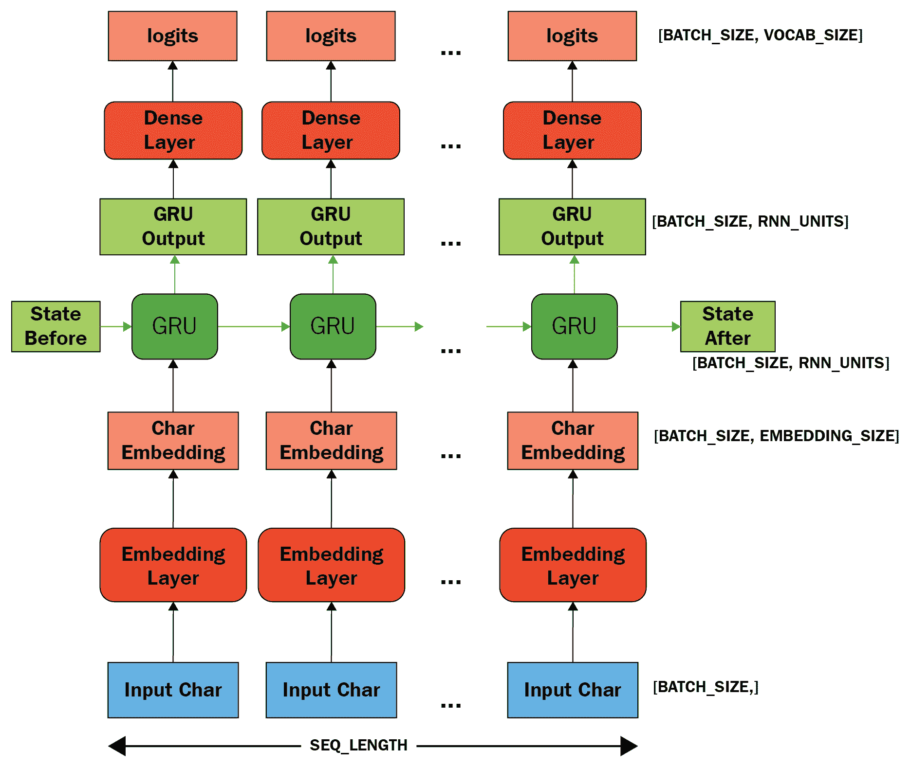 如下圖所示：  因此，實現此模型的代碼如下： ```py def build_model(vocabulary_size, embedding_dimension, recurrent_nn_units, batch_size): model = tf.keras.Sequential( [tf.keras.layers.Embedding(vocabulary_size, embedding_dimension, batch_input_shape=[batch_size, None]), recurrent_nn(recurrent_nn_units, return_sequences=True, recurrent_initializer='glorot_uniform', stateful=True), tf.keras.layers.Dense(vocabulary_length) ]) return model ``` 現在我們可以實例化我們的模型，如下所示： ```py model = build_model( vocabulary_size = len(vocabulary), embedding_dimension=embedding_dimension, recurrent_nn_units=recurrent_nn_units, batch_size=batch) ``` 現在，我們可以進行健全性檢查，以確保我們的模型輸出正確的形狀。 注意使用`dataset.take()`提取數據集的元素： ```py for batch_input_example, batch_target_example in dataset.take(1): batch_predictions_example = model(batch_input_example) print(batch_predictions_example.shape, "# (batch, sequence_length, vocabulary_length)") ``` 以下是此輸出： ```py (64, 100, 84) # (batch, sequence_length, vocabulary_length) ``` 這是預期的； 回想一下，我們的字符集中有`84`個唯一字符。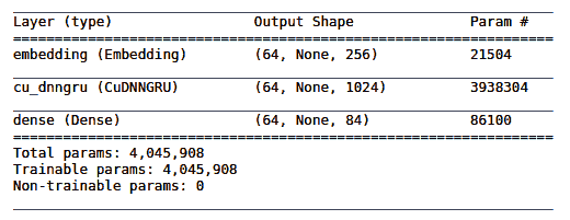 這是顯示我們的模型外觀的代碼： ```py model.summary() ``` 我們的模型架構摘要的輸出如下：  再次回想一下，我們有`84`輸入值，我們可以看到，對于嵌入層，`84 * 256 = 21,504`，對于密集層，`1024 * 84 + 84（偏置單元）= 86,100`。 # 使用我們的模型獲得預測 為了從我們的模型中獲得預測，我們需要從輸出分布中抽取一個樣本。 此采樣將為我們提供該輸出分布所需的字符（對輸出分布進行采樣很重要，因為像通常那樣對它進行`argmax`提取，很容易使模型陷入循環）。 在顯示索引之前，`tf.random.categorical`進行此采樣，`axis=-1`與`tf.squeeze`刪除張量的最后一個維度。 `tf.random.categorical`的簽名如下： ```py tf.random.categorical(logits, num_samples, seed=None, name=None, output_dtype=None) ``` 將其與調用進行比較，我們看到我們正在從預測（`example_batch_predictions[0]`）中獲取一個樣本（長度為`sequence_length = 100`）。 然后刪除了多余的尺寸，因此我們可以查找與示例相對應的字符： ```py sampled_indices = tf.random.categorical(logits=batch_predictions_example[0], num_samples=1) sampled_indices = tf.squeeze(sampled_indices,axis=-1).numpy() sampled_indices ``` 這將產生以下輸出： ```py array([79, 43, 3, 12, 20, 24, 54, 10, 61, 43, 46, 15, 0, 24, 39, 77, 2, 73, 4, 78, 5, 60, 13, 65, 1, 75, 47, 33, 61, 13, 64, 41, 32, 42, 40, 20, 37, 10, 60, 51, 21, 17, 69, 8, 3, 74, 64, 68, 2, 3, 35, 13, 67, 16, 46, 48, 47, 1, 38, 80, 47, 8, 32, 53, 50, 28, 63, 33, 35, 72, 80, 0, 7, 64, 2, 79, 1, 56, 61, 13, 55, 28, 62, 30, 40, 22, 32, 40, 27, 46, 21, 51, 10, 76, 64, 47, 72, 83, 45, 8]) ``` 讓我們看一下到訓練之前的一些輸入和輸出*：* ```py print("Input: \n", repr("".join(index_to_char[batch_input_example[0]]))) print("Next Char Predictions: \n", repr("".join(index_to_char[sampled_indices ]))) # ``` 因此輸出如下。 輸入的文本之后是下一個字符預測（在訓練之前）： ```py Input: 'r, that I might refer to it again; but I could not find it, and\nwas uneasy to think that it must hav' Next Char Predictions: "hFTzJe;rA?:G*'”x4d?&?ce9QekL:*O7@KuoZM&“$r0mg\n%/2-6QaE&$)/'Y8m.x)94b?fKp.rR?.3IMMTMjMMag.iL1LuM6 ?';" ``` 接下來，我們定義`loss`函數： ```py def loss(labels, logits): return tf.keras.losses.sparse_categorical_crossentropy(labels, logits, from_logits=True) ``` 然后，我們在訓練之前查看模型的損失，并進行另一次尺寸完整性檢查： ```py batch_loss_example = tf.compat.v1.losses.sparse_softmax_cross_entropy(batch_target_example, batch_predictions_example) print("Prediction shape: ", batch_predictions_example.shape, " # (batch_size, sequence_length, vocab_size)") print("scalar_loss: ", batch_loss_example.numpy()) ``` 這將產生以下輸出： ```py Prediction shape: (64, 100, 84) # (batch, sequence_length, vocabulary_length) scalar_loss: 4.429237 ``` 為了準備我們的訓練模型，我們現在使用`AdamOptimizer`和 softmax 交叉熵損失對其進行編譯： ```py #next produced by upgrade script.... #model.compile(optimizer = tf.compat.v1.train.AdamOptimizer(), loss = loss) #.... but following optimizer is available. model.compile(optimizer = tf.optimizers.Adam(), loss = loss) ``` 我們將保存模型的權重，因此，接下來，我們為此準備檢查點： ```py # The checkpoints will be saved in this directory directory = './checkpoints' # checkpoint files file_prefix = os.path.join(directory, "ckpt_{epoch}") callback=[tf.keras.callbacks.ModelCheckpoint(filepath=file_prefix, save_weights_only=True)] ``` 最后，我們可以使用對`model.fit()`的調用來訓練模型： ```py epochs=45 # *much* faster on GPU, ~10s / epoch, reduce this figure significantly if on CPU history = model.fit(dataset, epochs=epochs, steps_per_epoch=steps_per_epoch, callbacks=callback) ``` 這給出以下輸出： ```py Epoch 1/50 158/158 [==============================] - 10s 64ms/step - loss: 2.6995 .................... 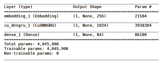Epoch 50/50 158/158 [==============================] - 10s 65ms/step - loss: 0.6143 ``` 以下是最新的檢查點： ```py tf.train.latest_checkpoint(directory) ``` 可以解決以下結果： ```py './checkpoints/ckpt_45' ``` 因此，我們可以重建模型（以展示其完成方式）： ```py model = build_model(vocabulary_size, embedding_dimension, recurrent_nn_units, batch_size=1) model.load_weights(tf.train.latest_checkpoint(directory)) model.build(tf.TensorShape([1, None])) model.summary() ``` 下表顯示了我們模型的摘要：  接下來，在給定訓練有素的模型，起始字符串和溫度的情況下，我們使用一個函數來生成新文本，其值確定文本的隨機性（低值給出更多可預測的文本；高值給出更多隨機的文本）。 首先，我們確定要生成的字符數，然后向量化起始字符串，并為其添加空白尺寸。 我們將額外的維添加到`input_string`變量中，因為 RNN 單元需要它（兩個必需的維是批量長度和序列長度）。 然后，我們初始化一個變量，用于存儲生成的文本。 `temperature`的值確定生成的文本的隨機性（較低的隨機性較小，意味著更可預測）。 在一個循環中，對于要生成的每個新字符，我們使用包含 RNN 狀態的模型來獲取下一個字符的預測分布。 然后使用多項式分布來找到預測字符的索引，然后將其用作模型的下一個輸入。 由于存在循環，模型返回的 RNN 狀態將反饋到模型中，因此它現在不僅具有一個字符，而且具有更多信息。 一旦預測了下一個字符，就將修改后的 RNN 狀態反復反饋到模型中，以便模型學習，因為它從先前預測的字符獲得的上下文會增加。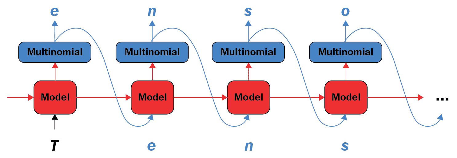 下圖顯示了它是如何工作的：  在這里，多項式用`tf.random.categorical`實現； 現在我們準備生成我們的預測文本： ```py def generate_text(model, start_string, temperature, characters_to_generate): # Vectorise the start string into numbers input_string = [char_to_index[char] for char in start_string] # add extra dimension to input_string input_string = tf.expand_dims(input_string, 0) # Empty list to store generated text generated = [] # (batch size is 1) model.reset_states() for i in range(characters_to_generate): predictions = model(input_string) #here's where we need the extra dimension # remove the batch dimension predictions = tf.squeeze(predictions, 0) # using a random categorical (multinomial) distribution to predict word returned by the model predictions = predictions / temperature predicted_id = tf.random.categorical(logits=predictions, num_samples=1)[-1,0].numpy() # Pass predicted word as next input to the model along with previous hidden state input_string = tf.expand_dims([predicted_id], 0) generated.append(index_to_char[predicted_id]) return (start_string + ''.join(generated)) # generated is a list ``` 因此，在定義函數之后，我們可以調用它以返回生成的文本。 在給定的函數參數中，低溫給出更多可預測的文本，而高溫給出更多隨機的文本。 同樣，您可以在此處更改起始字符串并更改函數生成的字符數： ```py generated_text = generate_text(model=model, start_string="Pip", temperature=0.1, characters_to_generate = 1000) print(generated_text) ``` 經過 30 個訓練周期后，將產生以下輸出： ```py Pip; it was a much better to and the Aged and weaking his hands of the windows of the way who went them on which the more I had been a very little for me, and I went on with his back in the soldiers of the room with the whole hand the other gentleman with the hand on the service, when I was a look of half of the room was was the first time of the money. I forgetter, Mr. Pip?” “I don't know that I have no more than I know what I have no inquiry with the rest of its being straight up again. He came out of the room, and in the midst of the room was was all the words, “and he came into the Castle. One would repeat it to your expectations condition of the courtyard. In a moment was the first time in the house to the fork, and we all lighted and at his being so beautiful looking at the convicts. My depression of the morning, I looked at him in the morning, I should not have been made a strong for the first time of the wall before the table to the forefinger of the room, and had not quite diffi ``` `Loss = 0.6761`； 該文本或多或少地被正確地拼寫和標點，盡管其含義（我們并未試圖實現）的含義在很大程度上是愚蠢的。 它還沒有學習如何正確使用語音標記。 只有兩個無意義的單詞（`forgetter`和`weaking`），經過檢查，在語義上仍然是合理的。 生成的是否為 Charles Dickens 風格是一個懸而未決的問題。 周期數的實驗表明，損失在約 45 周期時達到最小值，此后它開始增加。 45 個周期后，輸出如下： ```py Pip; or I should have felt painfully consciousness that he was the man with his back to the kitchen, and he seemed to have no strength, and as I had often seen her shutters with the poker on the parlor, through having been every disagreeable to be seen; I thought I would give him more letters of my own eyes and flared about the fire, and showed the greatest state of mind, I thought I would give up of his having fastened out of the room, and had made some advance in that respect to me to feel an indescribable awe as it was a to be even than ever of her steps, or for old asked, “Yes.” “What is it?” repeated Mr. Jaggers. “You know I was in my mind by his blue eyes most of all admirers, and that she had shaken hands contributing the poker out of his hands in his pockets and his dinner loosely tied in a busy preparation for the reference to my United and self-possession when Miss Havisham and Estella now that I had been too much to be the salvey dark night, which seemed so long ago. “Yes, de ``` `Loss = 0.6166`； 該模型現在似乎已正確配對了語音標記，并且沒有無意義的單詞。 # 總結 這樣就結束了我們對 RNN 的研究。 在本章中，我們首先討論了 RNN 的一般原理，然后介紹了如何獲取和準備一些供模型使用的文本，并指出在此處使用替代文本源很簡單。 然后，我們看到了如何創建和實例化我們的模型。 然后，我們訓練了模型并使用它從起始字符串中產生文本，并注意到網絡已了解到單詞是文本的單元以及如何拼寫各種各樣的單詞（有點像文本作者的風格）， 幾個非單詞。 在下一章中，我們將研究 TensorFlow Hub 的使用，它是一個軟件庫。